Text Sentiment Classification → Social Media Sentiment Tracking

Why RNN?

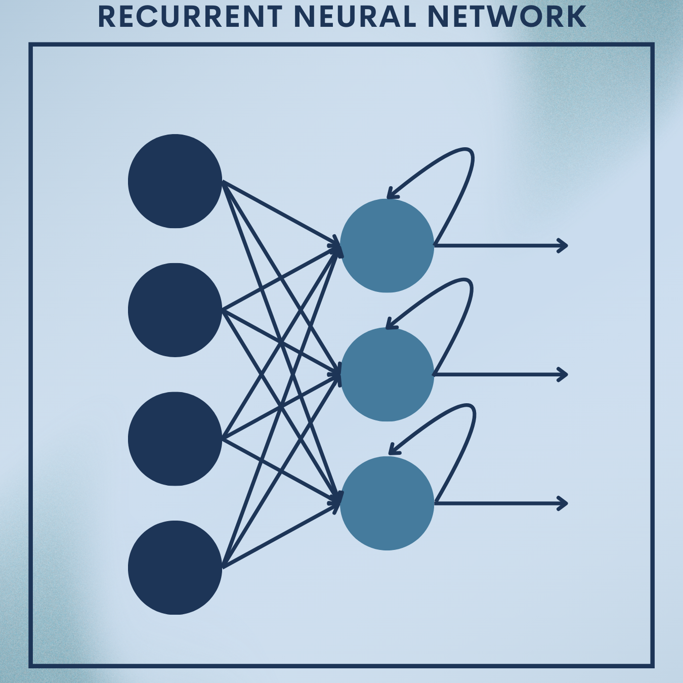
Customer reviews, tweets, and comments arrive as sequences of words where order matters. Recurrent Neural Networks (RNNs) give models memory, letting them read text left-to-right and build an internal summary before deciding whether a post feels positive or negative. In this tutorial you will:

Learn the theory behind vanilla RNNs and gated variants (GRU/LSTM), with clear math.
Build a sentiment classifier on a movie-review dataset as a toy problem.
Deploy it on a CSV of social posts to track brand sentiment over time, producing daily aggregates and simple alerts.

This module is designed for students, researchers, and engineers: theory that’s rigorous, plus production-ready code you can adapt.

Theory Deep Dive

1. Sequence modeling and notation

We observe a token sequence ${\mathbf{x}_1, \mathbf{x}_2, \ldots, \mathbf{x}_T}$ where each $\mathbf{x}_t \in \mathbb{R}^{V}$ is a one-hot vector over a vocabulary of size $V$ (in practice we use embeddings). The goal for sentiment is to map the entire sequence to a label $y \in {0,1}$ .

2. Vanilla RNN

At each time step, an RNN updates a hidden state $latex \mathbf{h}t \in \mathbb{R}^H$:
$latex \mathbf{h}t = \phi!\left(\mathbf{W}{xh}\mathbf{x}t + \mathbf{W}{hh}\mathbf{h}{t-1} + \mathbf{b}_h\right)$

Where $\phi$ is usually $\tanh$ or $\mathrm{ReLU}$ . For classification we use the final hidden state:
$\hat{y} = \sigma!\left(\mathbf{W}_{hy}\mathbf{h}_T + \mathbf{b}_y\right)$

Binary cross-entropy loss:
$\mathcal{L} = -\left[,y \log \hat{y} + (1-y)\log(1-\hat{y}),\right]$

3. Embeddings

Instead of one-hot inputs, we learn an embedding matrix $\mathbf{E} \in \mathbb{R}^{V \times d}$ so each token index $i$ maps to vector $\mathbf{e}_i \in \mathbb{R}^d$ . This reduces parameters and captures semantic similarity.

4. Backpropagation Through Time (BPTT)

Gradients flow through time by the chain rule:
$latex \frac{\partial \mathcal{L}}{\partial \mathbf{h}t} = \left(\prod{k=t+1}^{T} \mathbf{J}_k\right)\frac{\partial \mathcal{L}}{\partial \mathbf{h}_T}$
where $latex \mathbf{J}_k = \frac{\partial \mathbf{h}k}{\partial \mathbf{h}{k-1}}$. If the spectral radius of $\mathbf{J}_k$ is $<1$ , gradients vanish; if $>1$ , they explode. In practice we use gradient clipping and gated RNNs.

5. LSTM and GRU (gated RNNs)

Gates learn what to remember and forget.

GRU (Gated Recurrent Unit) (common, simpler):

Update gate $latex \mathbf{z}_t = \sigma(\mathbf{W}_z[\mathbf{x}t,\mathbf{h}{t-1}] + \mathbf{b}_z)$
Reset gate $latex \mathbf{r}_t = \sigma(\mathbf{W}_r[\mathbf{x}t,\mathbf{h}{t-1}] + \mathbf{b}_r)$
Candidate $latex \tilde{\mathbf{h}}_t = \tanh(\mathbf{W}_h[\mathbf{x}_t,, \mathbf{r}t \odot \mathbf{h}{t-1}] + \mathbf{b}_h)$
Hidden $latex \mathbf{h}_t = (1-\mathbf{z}t)\odot \mathbf{h}{t-1} + \mathbf{z}_t \odot \tilde{\mathbf{h}}_t$

LSTM maintains a cell state to mitigate vanishing gradients:

Input/forget/output gates $(\mathbf{i}_t,\mathbf{f}_t,\mathbf{o}_t)$ control cell $\mathbf{c}_t$ and hidden $\mathbf{h}_t$ . (Formulas omitted here for brevity but analogous.)

Either works well; we’ll implement a GRU classifier.

6. Practical concerns

Padding & masking: sequences vary in length; pad to max length and ensure the RNN ignores padding (PyTorch can use pack_padded_sequence, but we’ll keep fixed length for clarity).

Bidirectionality: read left-to-right and right-to-left to capture context; concatenate final states.

Regularization: dropout on embeddings and/or RNN outputs, $L_2$ weight decay, early stopping.

Optimization: Adam with learning rate in $[1\mathrm{e}{-4}, 1\mathrm{e}{-3}]$ , clip gradients (e.g., clip_grad_norm_ at 1.0).

Evaluation: accuracy and macro-F1; watch for class imbalance.

Baselines: logistic regression on bag-of-words; SVM; shallow CNN. RNNs often win when order matters.

Modern context: Transformers dominate long-range modeling, but RNNs remain compact, fast to train on small data, and easy to deploy.

Toy Problem – IMDB Movie-Review Sentiment

Goal: Train a binary sentiment classifier (positive/negative) on IMDB reviews, then evaluate.

Data Snapshot

(IMDB has 25k train / 25k test reviews, balanced.)

id	text (truncated)	label
1	“An amazing film with nuanced performances and a gripping narrative…”	1
2	“Boring and predictable. I wanted to like it, but it dragged on forever.”	0
3	“Beautiful cinematography; the plot is thin, yet the acting saves the day.”	1

Label mapping: 0 = negative, 1 = positive.

We’ll load this via the 🤗 datasets library for reliability and simplicity.

We’ll fine‑tune ResNet‑18 on a small ImageFolder dataset (e.g., dat to compute class weights to mitigate bias.

Step 1: Environment & imports

Environment & imports — install and import what we need.

This sets up core libraries for data loading, modeling, metrics, and progress bars.

# !pip install torch torchvision torchaudio datasets==2.* scikit-learn tqdm
import re, math, json, random, os
import torch, torch.nn as nn
from torch.utils.data import Dataset, DataLoader
from datasets import load_dataset
from sklearn.metrics import accuracy_score, f1_score
from tqdm import tqdm

Sets seeds for reproducibility and chooses GPU if available.

Step 2: Load IMDB and create splits

We fetch train/test splits from the IMDB dataset.

raw = load_dataset("imdb")  # returns {'train':..., 'test':...}
train_raw = raw["train"]
test_raw  = raw["test"]
len(train_raw), len(test_raw)

Step 3: Tokenizer and vocabulary

We define a simple regex tokenizer and build a frequency-filtered vocabulary. Unknowns map to <unk>. Sequences are padded/truncated to a fixed length (200).

def tokenize(text):
    text = text.lower()
    return re.findall(r"\b\w+\b", text)

# Build vocab from training data (limit size)
VOCAB_SIZE = 30000
min_freq   = 2
from collections import Counter
counter = Counter()
for ex in train_raw:
    counter.update(tokenize(ex["text"]))

# Keep tokens by frequency
itos = ["<pad>", "<unk>"]
itos += [w for (w,c) in counter.most_common(VOCAB_SIZE) if c >= min_freq and w not in ("<pad>","<unk>")]
stoi = {w:i for i,w in enumerate(itos)}
PAD_IDX, UNK_IDX = 0, 1

def numericalize(tokens, max_len=200):
    ids = [stoi.get(t, UNK_IDX) for t in tokens]
    ids = ids[:max_len]
    if len(ids) < max_len:
        ids = ids + [PAD_IDX]*(max_len - len(ids))
    return ids

Step 4: PyTorch Dataset & DataLoader

This wraps the HF dataset for PyTorch and creates shuffled mini-batches.

class TextDataset(Dataset):
    def __init__(self, hf_split, max_len=200):
        self.data = hf_split
        self.max_len = max_len
    def __len__(self):
        return len(self.data)
    def __getitem__(self, idx):
        ex = self.data[idx]
        tokens = tokenize(ex["text"])
        x = torch.tensor(numericalize(tokens, self.max_len), dtype=torch.long)
        y = torch.tensor(ex["label"], dtype=torch.float32)
        return x, y

max_len = 200
train_ds = TextDataset(train_raw, max_len=max_len)
test_ds  = TextDataset(test_raw,  max_len=max_len)

BATCH_SIZE = 128
train_loader = DataLoader(train_ds, batch_size=BATCH_SIZE, shuffle=True, num_workers=2)
test_loader  = DataLoader(test_ds,  batch_size=BATCH_SIZE, shuffle=False, num_workers=2)
len(train_ds), len(test_ds)

Step 5: Define the GRU sentiment classifier

We embed tokens, pass through a bidirectional GRU, and classify using the last hidden state(s).

class GRUSentiment(nn.Module):
    def __init__(self, vocab_size, embed_dim=128, hidden_dim=128, num_layers=1, bidirectional=True, dropout=0.3, pad_idx=0):
        super().__init__()
        self.bidirectional = bidirectional
        self.embedding = nn.Embedding(vocab_size, embed_dim, padding_idx=pad_idx)
        self.gru = nn.GRU(
            input_size=embed_dim,
            hidden_size=hidden_dim,
            num_layers=num_layers,
            batch_first=True,
            bidirectional=bidirectional,
            dropout=dropout if num_layers > 1 else 0.0
        )
        self.dropout = nn.Dropout(dropout)
        self.fc = nn.Linear(hidden_dim * (2 if bidirectional else 1), 1)

    def forward(self, x):
        # x: (B, T)
        emb = self.embedding(x)              # (B, T, E)
        out, h_n = self.gru(emb)             # h_n: (num_layers*num_directions, B, H)
        if self.bidirectional:
            # Concatenate last layer's forward & backward states
            h_f = h_n[-2,:,:]                # (B, H)
            h_b = h_n[-1,:,:]                # (B, H)
            h = torch.cat([h_f, h_b], dim=1) # (B, 2H)
        else:
            h = h_n[-1,:,:]                  # (B, H)
        h = self.dropout(h)
        logits = self.fc(h).squeeze(1)       # (B,)
        return logits

Step 6: Training loop

We optimize with Adam and BCEWithLogitsLoss, clip gradients to fight exploding gradients, and report accuracy/F1.

device = torch.device("cuda" if torch.cuda.is_available() else "cpu")
model = GRUSentiment(vocab_size=len(itos), embed_dim=128, hidden_dim=128, bidirectional=True, dropout=0.3, pad_idx=PAD_IDX).to(device)

optimizer = torch.optim.Adam(model.parameters(), lr=1e-3, weight_decay=1e-5)
criterion = nn.BCEWithLogitsLoss()

def evaluate(loader):
    model.eval()
    preds, golds = [], []
    with torch.no_grad():
        for xb, yb in loader:
            xb, yb = xb.to(device), yb.to(device)
            logits = model(xb)
            prob = torch.sigmoid(logits)
            pred = (prob >= 0.5).float()
            preds.append(pred.cpu())
            golds.append(yb.cpu())
    preds = torch.cat(preds).numpy()
    golds = torch.cat(golds).numpy()
    return accuracy_score(golds, preds), f1_score(golds, preds)

EPOCHS = 5
best_acc = 0.0
for epoch in range(1, EPOCHS+1):
    model.train()
    running_loss = 0.0
    for xb, yb in tqdm(train_loader, desc=f"Epoch {epoch}/{EPOCHS}"):
        xb, yb = xb.to(device), yb.to(device)
        optimizer.zero_grad()
        logits = model(xb)
        loss = criterion(logits, yb)
        loss.backward()
        nn.utils.clip_grad_norm_(model.parameters(), max_norm=1.0)
        optimizer.step()
        running_loss += loss.item() * xb.size(0)
    train_loss = running_loss / len(train_ds)
    acc, f1 = evaluate(test_loader)
    print(f"Epoch {epoch}: train_loss={train_loss:.4f} | test_acc={acc:.4f} | test_f1={f1:.4f}")

Step 7: Save artifacts (model + vocab)

We persist the trained model and vocabulary for later inference.

os.makedirs("artifacts", exist_ok=True)
torch.save(model.state_dict(), "artifacts/rnn_sentiment.pt")
with open("artifacts/vocab.json", "w") as f:
    json.dump({"itos": itos}, f)

Quick Reference: Full Code

# Train a GRU sentiment classifier on IMDB (compact)
# !pip install torch datasets scikit-learn tqdm
import re, json, os, torch, torch.nn as nn
from datasets import load_dataset
from collections import Counter
from torch.utils.data import Dataset, DataLoader
from sklearn.metrics import accuracy_score, f1_score

def tokenize(t): return re.findall(r"\b\w+\b", t.lower())
raw = load_dataset("imdb"); train_raw, test_raw = raw["train"], raw["test"]
counter = Counter(t for ex in train_raw for t in tokenize(ex["text"]))
itos = ["<pad>","<unk>"] + [w for w,c in counter.most_common(30000) if c>=2 and w not in ("<pad>","<unk>")]
stoi = {w:i for i,w in enumerate(itos)}; PAD_IDX, UNK_IDX = 0,1
def numericalize(tokens, L=200): 
    ids=[stoi.get(t,UNK_IDX) for t in tokens][:L]; return ids+[PAD_IDX]*(L-len(ids))
class TextDS(Dataset):
    def __init__(s, split): s.d=split
    def __len__(s): return len(s.d)
    def __getitem__(s,i):
        ex=s.d[i]; x=torch.tensor(numericalize(tokenize(ex["text"])),dtype=torch.long)
        y=torch.tensor(ex["label"],dtype=torch.float32); return x,y
train_ds, test_ds = TextDS(train_raw), TextDS(test_raw)
train_loader=DataLoader(train_ds, batch_size=128, shuffle=True, num_workers=2)
test_loader =DataLoader(test_ds,  batch_size=128, shuffle=False, num_workers=2)
class GRU(nn.Module):
    def __init__(s,V,E=128,H=128,bi=True,drop=0.3,pad=0):
        super().__init__(); s.bi=bi
        s.emb=nn.Embedding(V,E,padding_idx=pad)
        s.rnn=nn.GRU(E,H,batch_first=True,bidirectional=bi,dropout=drop if True else 0)
        s.do=nn.Dropout(drop); s.fc=nn.Linear(H*(2 if bi else 1),1)
    def forward(s,x):
        _,h=s.rnn(s.emb(x))
        h=torch.cat([h[-2],h[-1]],1) if s.bi else h[-1]; return s.fc(s.do(h)).squeeze(1)
device=torch.device("cuda" if torch.cuda.is_available() else "cpu")
model=GRU(len(itos)).to(device); opt=torch.optim.Adam(model.parameters(),lr=1e-3,weight_decay=1e-5)
crit=nn.BCEWithLogitsLoss()
def eval_(ldr):
    model.eval(); P,G=[],[]
    with torch.no_grad():
        for xb,yb in ldr:
            p=torch.sigmoid(model(xb.to(device))); P.append((p>=0.5).float().cpu()); G.append(yb)
    import torch as T; P=T.cat(P).numpy(); G=T.cat(G).numpy()
    return accuracy_score(G,P), f1_score(G,P)
for e in range(5):
    model.train()
    for xb,yb in train_loader:
        xb,yb=xb.to(device), yb.to(device)
        opt.zero_grad(); loss=crit(model(xb), yb); loss.backward()
        nn.utils.clip_grad_norm_(model.parameters(),1.0); opt.step()
    acc,f1=eval_(test_loader); print(e+1,acc,f1)
os.makedirs("artifacts",exist_ok=True)
torch.save(model.state_dict(),"artifacts/rnn_sentiment.pt")
with open("artifacts/vocab.json","w") as f: json.dump({"itos":itos},f)

Real‑World Application — Social Media Sentiment Tracking

Scenario: You receive a daily CSV export (posts.csv) with columns: created_at (ISO date), text, user_id. We’ll load the trained model, score each post, compute daily positive rates, and raise alerts when sentiment dips.

Step 1: Load artifacts and define the same preprocessing

We recreate the model and vocab exactly as trained to ensure token indices align.

import json, re, pandas as pd, torch, torch.nn as nn

with open("artifacts/vocab.json") as f:
    itos = json.load(f)["itos"]
stoi = {w:i for i,w in enumerate(itos)}
PAD_IDX, UNK_IDX = 0, 1

def tokenize(text): return re.findall(r"\b\w+\b", text.lower())
def numericalize(tokens, L=200):
    ids=[stoi.get(t,UNK_IDX) for t in tokens][:L]; return ids+[PAD_IDX]*(L-len(ids))

class GRUSentiment(nn.Module):
    def __init__(self, vocab_size, embed_dim=128, hidden_dim=128, bidirectional=True, dropout=0.3, pad_idx=0):
        super().__init__()
        self.bidirectional = bidirectional
        self.embedding = nn.Embedding(vocab_size, embed_dim, padding_idx=pad_idx)
        self.gru = nn.GRU(embed_dim, hidden_dim, batch_first=True, bidirectional=bidirectional)
        self.dropout = nn.Dropout(dropout)
        self.fc = nn.Linear(hidden_dim * (2 if bidirectional else 1), 1)
    def forward(self, x):
        _, h_n = self.gru(self.embedding(x))
        h = torch.cat([h_n[-2], h_n[-1]], 1) if self.bidirectional else h_n[-1]
        return self.fc(self.dropout(h)).squeeze(1)

device = torch.device("cuda" if torch.cuda.is_available() else "cpu")
model = GRUSentiment(vocab_size=len(itos)).to(device)
model.load_state_dict(torch.load("artifacts/rnn_sentiment.pt", map_location=device))
model.eval()

Step 2: Load posts, preprocess, and batch-infer

We score each post to get a positive probability and binary prediction.

import numpy as np
BATCH=256

df = pd.read_csv("posts.csv")  # columns: created_at, text, user_id
df["created_at"] = pd.to_datetime(df["created_at"]).dt.date

# Numericalize to tensors
def batch_predict(texts):
    X = [numericalize(tokenize(t)) for t in texts]
    X = torch.tensor(X, dtype=torch.long, device=device)
    with torch.no_grad():
        logits = model(X)
        probs  = torch.sigmoid(logits).cpu().numpy()
    return probs

probs = []
for i in range(0, len(df), BATCH):
    probs.extend(batch_predict(df["text"].iloc[i:i+BATCH].tolist()))
df["pos_prob"] = probs
df["pred"] = (df["pos_prob"] >= 0.5).astype(int)
df.head()

Step 3: Daily aggregation and simple alerting

We compute daily sentiment, a 3-day moving average, trigger alerts on dips, and save a CSV report for stakeholders.

daily = df.groupby("created_at").agg(
    total=("pred","size"),
    positives=("pred","sum"),
    mean_pos=("pos_prob","mean")
).reset_index()

# 3-day moving average of mean positive probability
daily["ma3"] = daily["mean_pos"].rolling(window=3, min_periods=1).mean()

# Alert when smoothed sentiment dips below 0.45
alerts = daily[daily["ma3"] < 0.45]
print("ALERT DAYS:\n", alerts[["created_at","ma3"]])
daily.to_csv("sentiment_daily_report.csv", index=False)

Step 4: (Optional) Quick Visualization

Generates a simple time-series chart you can drop into reports.

import matplotlib.pyplot as plt

plt.figure()
plt.plot(daily["created_at"], daily["mean_pos"], label="Daily mean positive prob")
plt.plot(daily["created_at"], daily["ma3"], label="3-day MA")
plt.xticks(rotation=45); plt.legend(); plt.title("Daily Social Sentiment"); plt.tight_layout()
plt.savefig("sentiment_daily_plot.png", dpi=150)

Quick Reference: Full Code

# Score posts.csv and produce daily report (compact)
import re, json, torch, torch.nn as nn, pandas as pd, numpy as np
with open("artifacts/vocab.json") as f: itos=json.load(f)["itos"]
stoi={w:i for i,w in enumerate(itos)}; PAD_IDX,UNK_IDX=0,1
def tok(t): return re.findall(r"\b\w+\b", t.lower())
def num(ts,L=200): 
    ids=[stoi.get(t,UNK_IDX) for t in ts][:L]; return ids+[PAD_IDX]*(L-len(ids))
class GRU(nn.Module):
    def __init__(s,V,E=128,H=128,bi=True,drop=0.3,pad=0):
        super().__init__(); s.bi=bi; s.emb=nn.Embedding(V,E,padding_idx=pad)
        s.rnn=nn.GRU(E,H,batch_first=True,bidirectional=bi); s.do=nn.Dropout(drop); s.fc=nn.Linear(H*(2 if bi else 1),1)
    def forward(s,x):
        _,h=s.rnn(s.emb(x)); h=torch.cat([h[-2],h[-1]],1) if s.bi else h[-1]; return s.fc(s.do(h)).squeeze(1)
dev=torch.device("cuda" if torch.cuda.is_available() else "cpu")
m=GRU(len(itos)).to(dev); m.load_state_dict(torch.load("artifacts/rnn_sentiment.pt", map_location=dev)); m.eval()
df=pd.read_csv("posts.csv"); df["created_at"]=pd.to_datetime(df["created_at"]).dt.date
B=256; P=[]
with torch.no_grad():
    for i in range(0,len(df),B):
        X=[num(tok(t)) for t in df["text"].iloc[i:i+B].tolist()]
        X=torch.tensor(X,dtype=torch.long,device=dev); P+=torch.sigmoid(m(X)).cpu().numpy().tolist()
df["pos_prob"]=P; df["pred"]=(df["pos_prob"]>=0.5).astype(int)
daily=df.groupby("created_at").agg(total=("pred","size"),positives=("pred","sum"),mean_pos=("pos_prob","mean")).reset_index()
daily["ma3"]=daily["mean_pos"].rolling(3, min_periods=1).mean()
daily.to_csv("sentiment_daily_report.csv",index=False)

Strengths & Limitations

Strengths

Order-aware modeling: Captures word order and local dependencies better than bag-of-words baselines.
Compact & efficient: Fewer parameters than many transformer models; fast to train on modest GPUs/CPUs.
Flexible: Works with variable lengths; bidirectional variants improve context capture.

Limitations

Long-range dependencies: Still struggles when crucial evidence is far apart; Transformers generally excel here.
Sequential computation: Harder to parallelize over time steps than CNNs/Transformers; slower on very long texts.
Vocabulary/OOV issues: Word-level models need careful handling of rare/unknown tokens; subword tokenization helps.

Final Notes

You built a full RNN pipeline: tokenization → vocabulary → padded tensors → GRU classifier → evaluation → saved artifacts → real-world inference and monitoring. You now own a lightweight, explainable sentiment system that can run on small machines and be embedded in dashboards or alerting workflows.

This approach often suffices for many production-adjacent analytics where speed, simplicity, and cost matter.

Next Steps for You:

Upgrade the model:

Try LSTM or stacked/bidirectional RNNs; tune $d, H$ , dropout, and learning rate.
Use pretrained embeddings (GloVe/fastText) to improve performance on small data.

Productionize the pipeline:

Export to TorchScript or ONNX; wrap in a simple FastAPI service.
Add evaluation dashboards, threshold calibration (maximize F1), and A/B tests against baselines.

Improve text handling (optional):

Move to subword tokenization (e.g., SentencePiece/BPE) to reduce OOVs.
Add domain adaptation: fine-tune on your own labeled social data.

References

[1] Y. Goldberg, Neural Network Methods for Natural Language Processing. Morgan & Claypool, 2017.
[2] S. Hochreiter and J. Schmidhuber, “Long Short-Term Memory,” Neural Computation, vol. 9, no. 8, pp. 1735–1780, 1997.
[3] K. Cho et al., “Learning Phrase Representations using RNN Encoder–Decoder for Statistical Machine Translation,” EMNLP, 2014.
[4] T. Mikolov et al., “Recurrent neural network based language model,” INTERSPEECH, 2010.
[5] I. Goodfellow, Y. Bengio, and A. Courville, Deep Learning. MIT Press, 2016.
[6] A. Maas et al., “Learning Word Vectors for Sentiment Analysis,” ACL, 2011 (IMDB dataset).
[7] D. Jurafsky and J. H. Martin, Speech and Language Processing, 3rd ed. Draft, 2023.
[8] C. Olah, “Understanding LSTM Networks,” colah’s blog, 2015.
[9] A. Karpathy, “The Unreasonable Effectiveness of Recurrent Neural Networks,” 2015.
[10] J. Howard and S. Ruder, “Universal Language Model Fine-tuning for Text Classification,” ACL, 2018.

Recurrent Neural Networks (RNNs): Memory for Language

Why RNN?

Theory Deep Dive

1. Sequence modeling and notation

2. Vanilla RNN

3. Embeddings

4. Backpropagation Through Time (BPTT)

5. LSTM and GRU (gated RNNs)

6. Practical concerns

Toy Problem – IMDB Movie-Review Sentiment

Data Snapshot

Step 1: Environment & imports

Step 2: Load IMDB and create splits

Step 3: Tokenizer and vocabulary

Step 4: PyTorch Dataset & DataLoader

Step 5: Define the GRU sentiment classifier

Step 6: Training loop

Step 7: Save artifacts (model + vocab)

Quick Reference: Full Code

Real‑World Application — Social Media Sentiment Tracking

Step 1: Load artifacts and define the same preprocessing

Step 2: Load posts, preprocess, and batch-infer

Step 3: Daily aggregation and simple alerting

Step 4: (Optional) Quick Visualization

Quick Reference: Full Code

Strengths & Limitations

Strengths

Limitations

Final Notes

References

Leave a comment Cancel reply

Recurrent Neural Networks (RNNs): Memory for Language

Why RNN?

Theory Deep Dive

1. Sequence modeling and notation

2. Vanilla RNN

3. Embeddings

4. Backpropagation Through Time (BPTT)

5. LSTM and GRU (gated RNNs)

6. Practical concerns

Toy Problem – IMDB Movie-Review Sentiment

Data Snapshot

Step 1: Environment & imports

Step 2: Load IMDB and create splits

Step 3: Tokenizer and vocabulary

Step 4: PyTorch Dataset & DataLoader

Step 5: Define the GRU sentiment classifier

Step 6: Training loop

Step 7: Save artifacts (model + vocab)

Quick Reference: Full Code

Real‑World Application — Social Media Sentiment Tracking

Step 1: Load artifacts and define the same preprocessing

Step 2: Load posts, preprocess, and batch-infer

Step 3: Daily aggregation and simple alerting

Step 4: (Optional) Quick Visualization

Quick Reference: Full Code

Strengths & Limitations

Strengths

Limitations

Final Notes

References

Share this:

Leave a comment Cancel reply