
MNIST Handwritten Digits → Bank Check Digit Recognition
Why this concept matters
Feedforward neural networks (a.k.a. multilayer perceptrons, MLPs) are the canonical “hello world” of deep learning. Despite their simplicity, they power practical systems where inputs are fixed‑length vectors: OCR for digits, fraud flags from tabular features, or sensor‑based fault detection. In this lesson you’ll:
- Train a feedforward network to classify MNIST handwritten digits.
- Understand the math of forward propagation, softmax, cross‑entropy, and backpropagation.
- Build a small OCR pipeline that reads a numeric amount from a cropped bank check image.
This module is a bridge from classic ML to deep learning: you’ll see why MLPs work, where they struggle (images!), and why CNNs came next.
From Perceptron to Multilayer Networks (A Brief History)
Where we came from. The perceptron (Rosenblatt, 1957–58) gave us a trainable single neuron that linearly separates two classes. But single layers can’t model non-linear decision boundaries (e.g., XOR), as shown by Minsky & Papert (1969). Research cooled until the 1980s, when two developments reignited the field:
- Multi-Layer Perceptrons (MLPs): Stack neurons into layers and insert non-linear activations between linear transforms. This lets the model carve complex, curved decision regions.
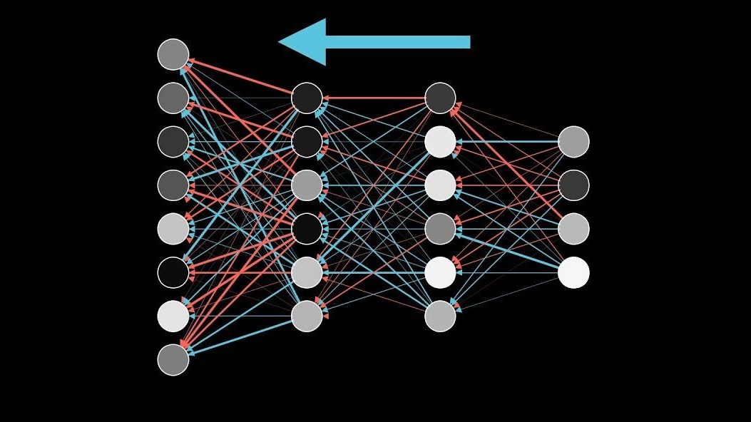
- Backpropagation (Rumelhart, Hinton, Williams, 1986): An efficient way to compute gradients layer-by-layer using the chain rule, enabling practical training of deeper models.
Other threads you’ll see referenced in histories:
- McCulloch–Pitts neurons (1943): Abstract “threshold logic units,” the ancestor of perceptrons.
- GMDH (Ivakhnenko, 1965): Early layered models with polynomial units—an MLP-like idea for nonlinearity.
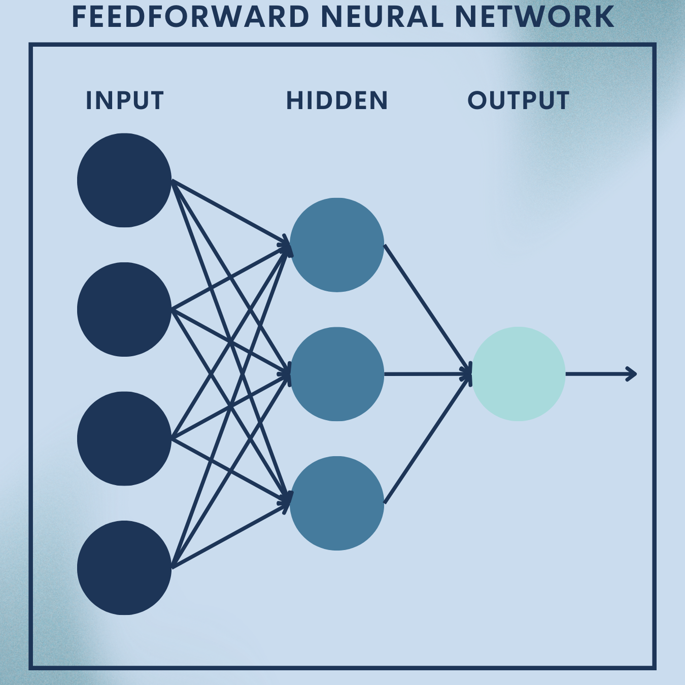
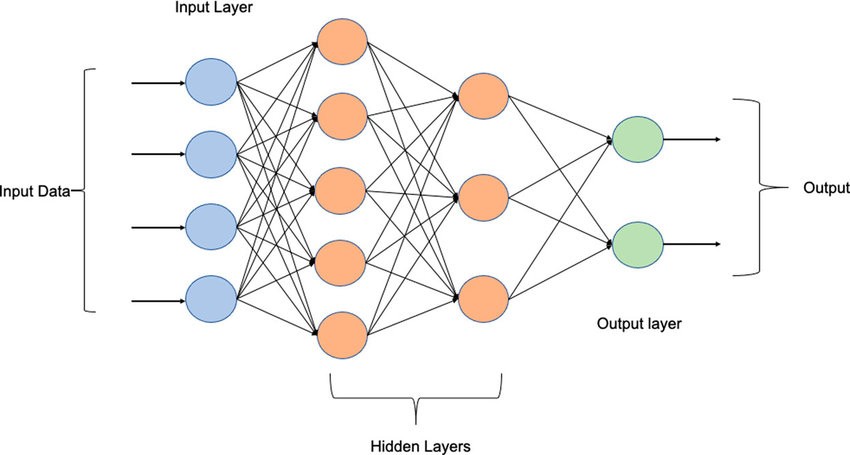
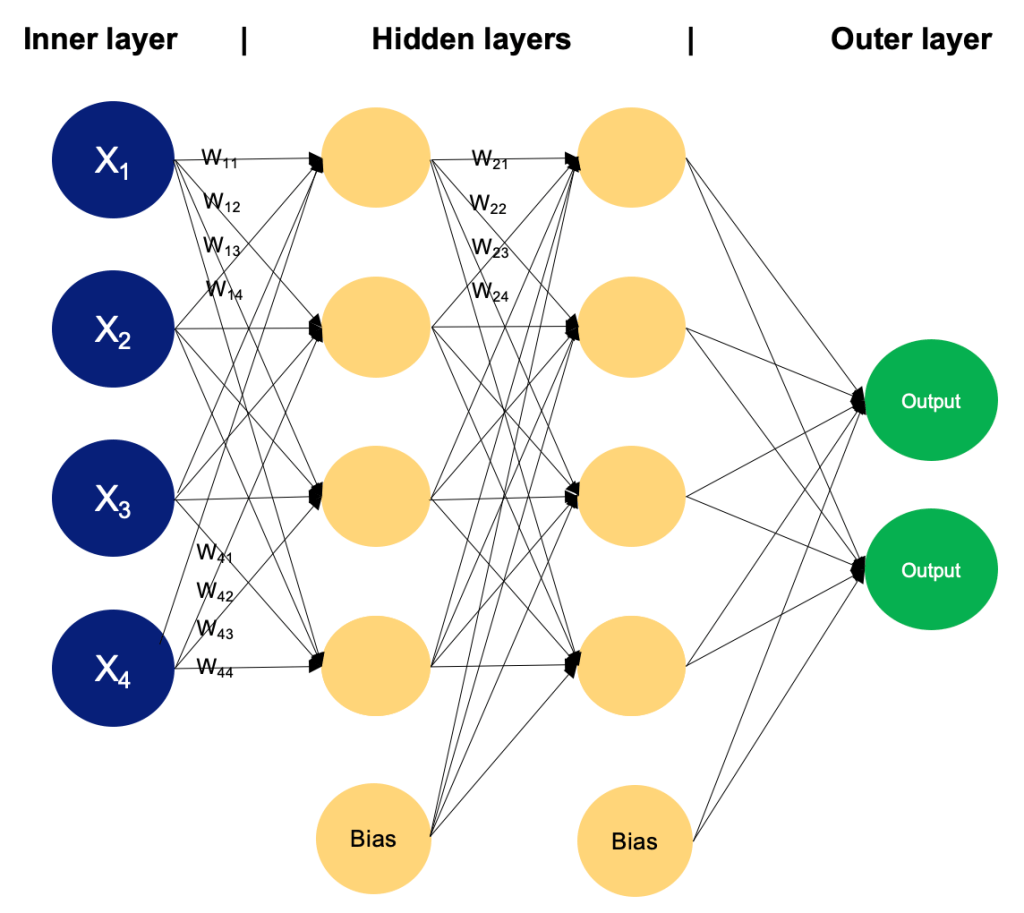
Today’s framing. An MLP / Feedforward Neural Network is the simplest deep architecture: information flows one way (no cycles), layer by layer, from inputs to outputs. It remains the workhorse for fixed-length vectors (tabular features, embeddings, sensor summaries), and a pedagogical bridge to CNNs/RNNs/Transformers.
Theory Deep Dive
Anatomy and Data Flow (Forward Pass Intuition)
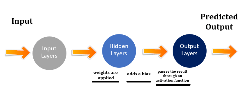
An MLP composes affine transforms and non-linear activations:
- Input layer: fixed-length feature vector
.
- Hidden layers (
): each computes a pre-activation and activation
with.
- Output layer (
): for multiclass classification, apply softmax to logits
to get class probabilities.


What changed vs. a perceptron? We no longer fit just one hyperplane. Stacking layers with nonlinearity builds hierarchical features: later layers recombine earlier ones into progressively more discriminative abstractions.
Building Blocks (Components You’ll Always See)
- Neurons/Units: Minimal compute cells applying
then
.
- Weights
& Biases
: Learned parameters.
- Activations
- Loss function: Measures prediction error (e.g., cross-entropy).
- Optimizer: Adjusts parameters by descending the loss surface using gradients (SGD/Adam).
- Regularizers: Stabilize training and improve generalization (L2, dropout, early stopping, batch norm).
Common Activations at a Glance
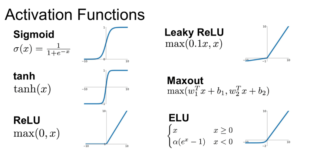
| Activation | Formula | Pros | Cautions |
| ReLU |  | Fast, sparse, stable deep training | “Dead” units if learning rate too high |
| Leaky ReLU |  | Fixes dead units | Slight extra hyperparam ( ) ) |
| Tanh |  | Zero-centered, smooth | Saturates (vanishing gradients) |
| Sigmoid |  | Probabilistic interpretation | Saturation + not zero-centered |
For hidden layers in MLPs, ReLU/Leaky ReLU are strong defaults. For outputs: softmax (multiclass), sigmoid (multi-label), or identity (regression).
Training Mechanics (Backprop Without Tears)
Forward pass: compute logits/probabilities for a batch.
Loss: for one-hot label 


Backward pass: use the chain rule to accumulate gradients from output → input:
- Softmax-CE trick:
- Then per layer, propagate through
,
, and the activation derivative (e.g., ReLU gate
).
- Update parameters via SGD/Adam.

Why it works: backprop reuses intermediate results (the 

Where MLPs Shine—and Where They Struggle
Strengths (use them when):
- Inputs are fixed-length vectors (tabular features, embeddings from upstream encoders).
- You want universal approximation power: with enough width, MLPs approximate continuous functions on compact sets.
- You need a simple, robust baseline for structured data (credit scoring, churn, fraud flags, sensor fault detection).
Limitations on images/sequences:
- MLPs ignore spatial locality (neighboring pixels) and translation invariance; they require many parameters for vision.
- They have no memory; each input is processed independently (no recurrence/attention).
Toy Problem – MNIST Handwritten Digit Recognition
Goal: Classify $28\times 28$ grayscale digits (0–9).
Data Snapshot
MNIST contains 60,000 training and 10,000 test images; classes are roughly balanced.
| Split | Samples | Image size | Channels | Classes |
|---|---|---|---|---|
| Train | 60,000 | 28×28 | 1 | 10 (digits 0–9) |
| Test | 10,000 | 28×28 | 1 | 10 |
We’ll flatten each image to a 784‑dim vector and feed it to an MLP.
Step 1: Setup
Install and import packages.
import torch, torch.nn as nn, torch.nn.functional as F
from torch.utils.data import DataLoader
from torchvision import datasets, transforms
import matplotlib.pyplot as plt
from sklearn.metrics import confusion_matrix, classification_report
import numpy as np
import itertools, time

device = torch.device('cuda' if torch.cuda.is_available() else 'cpu')
print('Device:', device)
Creates the environment and selects GPU if available.
Step 2: Load & normalize MNIST
Loads MNIST and applies standard normalization for faster, stable training.
transform = transforms.Compose([
    transforms.ToTensor(),
    transforms.Normalize((0.1307,), (0.3081,))  # mean/std for MNIST
])

train_ds = datasets.MNIST(root='./data', train=True, download=True, transform=transform)
test_ds  = datasets.MNIST(root='./data', train=False, download=True, transform=transform)

train_loader = DataLoader(train_ds, batch_size=128, shuffle=True, num_workers=2)
test_loader  = DataLoader(test_ds, batch_size=256, shuffle=False, num_workers=2)
len(train_ds), len(test_ds)
Step 3: Peek at the data
Visual sanity check: a grid of random digits.
images, labels = next(iter(train_loader))
fig, axes = plt.subplots(2, 6, figsize=(9,3))
for ax, img, lbl in zip(axes.ravel(), images[:12], labels[:12]):
    ax.imshow(img.squeeze().numpy(), cmap='gray')
    ax.set_title(int(lbl))
    ax.axis('off')
plt.tight_layout(); plt.show()
Step 4: Define the MLP model
Two hidden layers with ReLU + Dropout; He initialization for stable ReLU training.
class MLP(nn.Module):
    def __init__(self):
        super().__init__()
        self.net = nn.Sequential(
            nn.Flatten(),                  # 28x28 -> 784
            nn.Linear(784, 256),
            nn.ReLU(),
            nn.Dropout(0.2),
            nn.Linear(256, 128),
            nn.ReLU(),
            nn.Dropout(0.2),
            nn.Linear(128, 10)            # logits
        )
        self.apply(self._init)
    def _init(self, m):
        if isinstance(m, nn.Linear):
            nn.init.kaiming_normal_(m.weight, nonlinearity='relu')
            nn.init.zeros_(m.bias)
    def forward(self, x):
        return self.net(x)

model = MLP().to(device)
print(model)
Step 5: Train
Optimizes cross‑entropy using Adam for 5 epochs with weight decay.
optimizer = torch.optim.Adam(model.parameters(), lr=1e-3, weight_decay=1e-4)  # L2 via weight_decay
criterion = nn.CrossEntropyLoss()

def train_one_epoch(epoch):
    model.train(); running_loss, correct, total = 0.0, 0, 0
    for x, y in train_loader:
        x, y = x.to(device), y.to(device)
        optimizer.zero_grad()
        logits = model(x)
        loss = criterion(logits, y)
        loss.backward()
        optimizer.step()
        running_loss += loss.item() * x.size(0)
        pred = logits.argmax(dim=1)
        correct += (pred == y).sum().item()
        total += y.size(0)
    print(f"Epoch {epoch}: loss={(running_loss/total):.4f}, acc={(correct/total):.4f}")

for epoch in range(1, 6):
    train_one_epoch(epoch)
Step 6: Evaluate on test set
Reports the overall accuracy on 10,000 test images. An MLP typically reaches \~97–98%.
model.eval(); correct, total = 0, 0
all_preds, all_labels = [], []
with torch.no_grad():
    for x, y in test_loader:
        x, y = x.to(device), y.to(device)
        logits = model(x)
        preds = logits.argmax(dim=1)
        correct += (preds == y).sum().item()
        total += y.size(0)
        all_preds.append(preds.cpu())
        all_labels.append(y.cpu())

test_acc = correct/total
all_preds = torch.cat(all_preds).numpy(); all_labels = torch.cat(all_labels).numpy()
print('Test accuracy:', round(test_acc, 4))
(Optional) Confusion matrix and per‑class metrics:’
Shows where the model confuses visually similar digits (e.g., 4 vs 9, 3 vs 5).
cm = confusion_matrix(all_labels, all_preds)
print(classification_report(all_labels, all_preds, digits=4))
Step 7: Save & single‑image inference
Saves the model and demonstrates prediction with softmax confidence.
PATH = 'mnist_mlp.pt'
torch.save(model.state_dict(), PATH)

# Single image inference demo
model2 = MLP().to(device)
model2.load_state_dict(torch.load(PATH, map_location=device))
model2.eval()

x, y = test_ds[0]
with torch.no_grad():
    logits = model2(x.unsqueeze(0).to(device))
    prob = F.softmax(logits, dim=1).cpu().numpy().squeeze()
    pred = prob.argmax()
print('True:', y, 'Pred:', pred, 'Confidence:', f"{prob[pred]:.3f}")
Quick Reference: Full Code
import torch, torch.nn as nn, torch.nn.functional as F
from torch.utils.data import DataLoader
from torchvision import datasets, transforms

device = torch.device('cuda' if torch.cuda.is_available() else 'cpu')

train_loader = DataLoader(datasets.MNIST('./data', True, download=True,
    transform=transforms.Compose([transforms.ToTensor(), transforms.Normalize((0.1307,), (0.3081,))])),
    batch_size=128, shuffle=True)

test_loader = DataLoader(datasets.MNIST('./data', False, download=True,
    transform=transforms.Compose([transforms.ToTensor(), transforms.Normalize((0.1307,), (0.3081,))])),
    batch_size=256, shuffle=False)

class MLP(nn.Module):
    def __init__(self):
        super().__init__(); self.f = nn.Sequential(
            nn.Flatten(), nn.Linear(784,256), nn.ReLU(), nn.Dropout(0.2),
            nn.Linear(256,128), nn.ReLU(), nn.Dropout(0.2), nn.Linear(128,10))
        self.apply(lambda m: nn.init.kaiming_normal_(m.weight) if isinstance(m,nn.Linear) else None)
    def forward(self,x): return self.f(x)

model = MLP().to(device); opt = torch.optim.Adam(model.parameters(), lr=1e-3, weight_decay=1e-4)
crit = nn.CrossEntropyLoss()
for _ in range(5):
    model.train()
    for x,y in train_loader:
        x,y=x.to(device),y.to(device); opt.zero_grad(); loss=crit(model(x),y); loss.backward(); opt.step()

model.eval(); correct=tot=0
with torch.no_grad():
    for x,y in test_loader:
        p=model(x.to(device)).argmax(1).cpu(); correct+=(p==y).sum().item(); tot+=y.size(0)
print('Test acc:', correct/tot)
Real‑World Application — Bank Check Digit Recognition (OCR)
Scenario. You have a cropped image of a numeric field on a bank check (e.g., amount or account digits). We’ll segment digits, normalize them to MNIST format, and classify with the trained MLP.
Note: Production OCR for checks typically uses the MICR E13B or CMC‑7 fonts and robust CNNs. Here we keep an educational, MLP‑based pipeline.
Step 1: Preprocessing & segmentation
We’ll use OpenCV to binarize the image and extract digit contours from left‑to‑right.
import cv2, numpy as np, torch
import torch.nn.functional as F

# Load trained model
model = MLP().to(device)
model.load_state_dict(torch.load('mnist_mlp.pt', map_location=device))
model.eval()

# Load a cropped grayscale image containing a sequence of digits (e.g., 'check_amount.png')
img = cv2.imread('check_amount.png', cv2.IMREAD_GRAYSCALE)

# 1) Denoise & binarize (Otsu)
blur = cv2.GaussianBlur(img, (3,3), 0)
_, bw = cv2.threshold(blur, 0, 255, cv2.THRESH_BINARY_INV + cv2.THRESH_OTSU)

# 2) Morphology to clean small noise
kernel = cv2.getStructuringElement(cv2.MORPH_RECT, (2,2))
bw = cv2.morphologyEx(bw, cv2.MORPH_OPEN, kernel, iterations=1)

# 3) Find contours and bounding boxes
cnts, _ = cv2.findContours(bw, cv2.RETR_EXTERNAL, cv2.CHAIN_APPROX_SIMPLE)
boxes = [cv2.boundingRect(c) for c in cnts]
# Filter by reasonable size (tune thresholds for your images)
boxes = [b for b in boxes if 8 <= b[2] <= 80 and 12 <= b[3] <= 100]
boxes = sorted(boxes, key=lambda b: b[0])  # left-to-right
Binarizes and isolates candidate digit blobs; sorts them by x‑coordinate.
Step 2: Normalize each glyph to MNIST‑like 28×28
Resizes each contour to a 20‑pixel box and centers it on a 28×28 canvas (MNIST convention).
def to_mnist_patch(gray, box):
    x,y,w,h = box
    digit = gray[y:y+h, x:x+w]
    # Resize the longest side to 20px keeping aspect ratio
    scale = 20.0 / max(w,h)
    resized = cv2.resize(digit, (max(1,int(w*scale)), max(1,int(h*scale))), interpolation=cv2.INTER_AREA)
    # Place into a 28x28 canvas
    canvas = np.zeros((28,28), dtype=np.uint8)
    offx = (28 - resized.shape[1]) // 2
    offy = (28 - resized.shape[0]) // 2
    canvas[offy:offy+resized.shape[0], offx:offx+resized.shape[1]] = resized
    # Center via center-of-mass shift (optional)
    cy, cx = nd_center_of_mass(canvas)
    shiftx, shifty = int(round(14 - cx)), int(round(14 - cy))
    M = np.float32([[1,0,shiftx],[0,1,shifty]])
    canvas = cv2.warpAffine(canvas, M, (28,28))
    return canvas

from scipy.ndimage import center_of_mass as nd_center_of_mass

patches = [to_mnist_patch(bw, b) for b in boxes]
Step 3: Classify each digit and assemble the string
Runs each 28×28 patch through the MLP; concatenates predictions into a number string.
def predict_digit(patch28):
    # MNIST normalization: scale to [0,1], then normalize with dataset mean/std
    x = torch.tensor(patch28/255.0, dtype=torch.float32).unsqueeze(0).unsqueeze(0)
    x = (x - 0.1307) / 0.3081
    with torch.no_grad():
        logits = model(x.to(device))
        prob = F.softmax(logits, dim=1).cpu().numpy().squeeze()
        return int(prob.argmax()), float(prob.max())

preds = [predict_digit(p) for p in patches]
recognized = ''.join(str(d) for d,_ in preds)
print('Recognized digits:', recognized)
Step 4: (Optional) Simple checksum sanity check
Some institutions use checksums for numeric identifiers. As a placeholder, here’s **Luhn** (common for cards, not checks) to illustrate the idea.
def luhn_ok(num_str: str) -> bool:
    digits = [int(c) for c in num_str if c.isdigit()][::-1]
    s = 0
    for i,d in enumerate(digits):
        if i % 2 == 1:
            d = d*2
            if d > 9: d -= 9
        s += d
    return s % 10 == 0

print('Luhn valid?', luhn_ok(recognized))
Demonstrates post‑processing; replace with your bank’s actual checksum rule if applicable.
Quick Reference: Bank‑check OCR (compact)
# Needs: trained MLP saved as 'mnist_mlp.pt', OpenCV, SciPy
import cv2, numpy as np, torch, torch.nn as nn, torch.nn.functional as F
from scipy.ndimage import center_of_mass

class MLP(nn.Module):
    def __init__(self):
        super().__init__(); self.f = nn.Sequential(
            nn.Flatten(), nn.Linear(784,256), nn.ReLU(), nn.Dropout(0.2),
            nn.Linear(256,128), nn.ReLU(), nn.Dropout(0.2), nn.Linear(128,10))
        self.apply(lambda m: nn.init.kaiming_normal_(m.weight) if isinstance(m,nn.Linear) else None)
    def forward(self,x): return self.f(x)

model = MLP(); model.load_state_dict(torch.load('mnist_mlp.pt', map_location='cpu')); model.eval()

def preprocess(img_path):
    g = cv2.imread(img_path, 0)
    g = cv2.GaussianBlur(g, (3,3), 0)
    _, bw = cv2.threshold(g, 0, 255, cv2.THRESH_BINARY_INV+cv2.THRESH_OTSU)
    bw = cv2.morphologyEx(bw, cv2.MORPH_OPEN, cv2.getStructuringElement(cv2.MORPH_RECT,(2,2)),1)
    cnts,_ = cv2.findContours(bw, cv2.RETR_EXTERNAL, cv2.CHAIN_APPROX_SIMPLE)
    boxes = sorted([cv2.boundingRect(c) for c in cnts if 8<=cv2.boundingRect(c)[2]<=80 and 12<=cv2.boundingRect(c)[3]<=100], key=lambda b:b[0])
    return bw, boxes

def to_patch(bw, box):
    x,y,w,h = box
    d = bw[y:y+h, x:x+w]
    s = 20.0/max(w,h)
    r = cv2.resize(d, (max(1,int(w*s)), max(1,int(h*s))), interpolation=cv2.INTER_AREA)
    c = np.zeros((28,28), np.uint8)
    ox, oy = (28-r.shape[1])//2, (28-r.shape[0])//2
    c[oy:oy+r.shape[0], ox:ox+r.shape[1]] = r
    cy,cx = center_of_mass(c)
    M = np.float32([[1,0,int(round(14-cx))],[0,1,int(round(14-cy))]])
    return cv2.warpAffine(c, M, (28,28))

def predict_patch(p):
    x = torch.tensor(p/255.0, dtype=torch.float32).unsqueeze(0).unsqueeze(0)
    x = (x-0.1307)/0.3081
    with torch.no_grad():
        return model(x).argmax(1).item()

def recognize(img_path):
    bw, boxes = preprocess(img_path)
    digits = [predict_patch(to_patch(bw,b)) for b in boxes]
    return ''.join(map(str, digits))

print('Recognized:', recognize('check_amount.png'))
Strengths & Limitations
Strengths
- Simple, fast baseline for fixed‑size inputs; easy to implement and debug.
- Universal approximator with sufficient width; effective on tabular data.
- Works well on MNIST without specialized layers (~97–98% accuracy).
Limitations
- Ignores spatial structure of images; lacks translation/rotation invariance.
- Parameter‑heavy on high‑dimensional inputs; prone to overfitting without regularization.
- Typically outperformed by CNNs on real‑world OCR and vision tasks.
Final Notes
You built and understood an MLP end‑to‑end: forward pass, softmax, cross‑entropy, backprop, initialization, and regularization. You trained a solid MNIST classifier and turned it into a practical OCR pipeline for a bank‑check‑like image.
This foundation equips you to reason about deeper architectures (CNNs/RNNs/Transformers) because the same core ideas—composing differentiable functions and optimizing with gradient descent—carry forward.
Next Steps for You:
Upgrade to CNNs (e.g., LeNet, ResNet‑style blocks) for translation‑invariant, higher‑accuracy digit recognition.
Data augmentation (affine transforms, elastic distortions) to improve robustness to writing style, rotation, and noise.
Explore learning‑rate schedules (cosine decay, one‑cycle) and BatchNorm to speed convergence.
Try quantization/pruning for edge deployment on low‑power devices.
References
[1] D. E. Rumelhart, G. E. Hinton, and R. J. Williams, “Learning representations by back‑propagating errors,” Nature, vol. 323, pp. 533–536, 1986.
[2] Y. LeCun, L. Bottou, Y. Bengio, and P. Haffner, “Gradient‑based learning applied to document recognition,” Proceedings of the IEEE, vol. 86, no. 11, pp. 2278–2324, 1998.
[3] Y. LeCun, C. Cortes, and C. J. C. Burges, “The MNIST database of handwritten digits,” 2010. [Online]. Available: http://yann.lecun.com/exdb/mnist/
[4] X. Glorot and Y. Bengio, “Understanding the difficulty of training deep feedforward neural networks,” in Proc. AISTATS, 2010.
[5] K. He, X. Zhang, S. Ren, and J. Sun, “Delving deep into rectifiers: Surpassing human‑level performance on ImageNet classification,” in Proc. ICCV, 2015.
[6] G. Hinton, N. Srivastava, A. Krizhevsky, I. Sutskever, and R. Salakhutdinov, “Improving neural networks by preventing co‑adaptation of feature detectors,” 2012. (Dropout arXiv preprint; later formalized in 2014.)
[7] D. P. Kingma and J. Ba, “Adam: A method for stochastic optimization,” in Proc. ICLR, 2015.
[8] S. Ioffe and C. Szegedy, “Batch Normalization: Accelerating deep network training by reducing internal covariate shift,” in Proc. ICML, 2015.
[9] I. Goodfellow, Y. Bengio, and A. Courville, Deep Learning. MIT Press, 2016.
[10] V. Nair and G. Hinton, “Rectified linear units improve restricted Boltzmann machines,” in Proc. ICML, 2010.

Leave a comment