CIFAR-10 Image Classification → Manufacturing Defect Detection

Why CNNs?

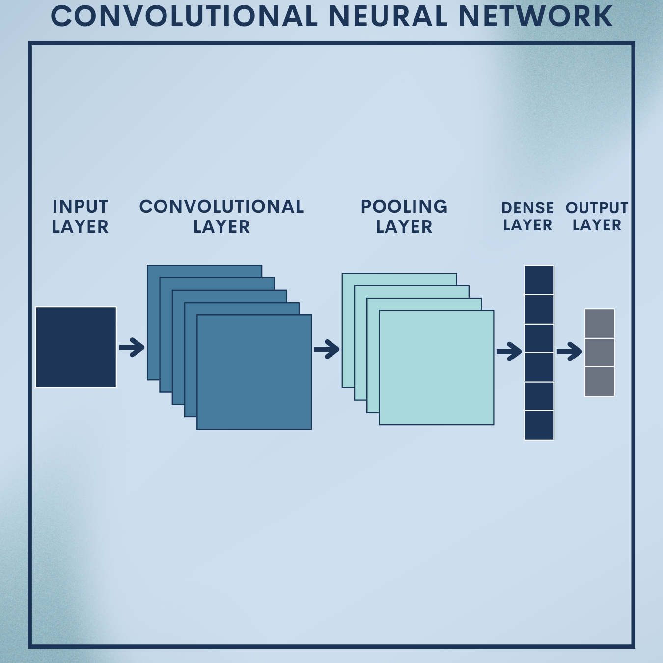
If your data is made of pixels—product photos, x-rays, traffic cameras, satellite images—CNNs are the workhorse that turn raw images into decisions. They learn what to look for (edges, textures, parts, objects) directly from data, eliminating brittle hand-crafted features. In this tutorial, you’ll:

Train a CNN from scratch on CIFAR-10 (toy but realistic).
Apply transfer learning to a manufacturing setting to flag defective vs. OK items.
Learn the theory deeply enough to reason about architecture, receptive fields, invariances, optimization, and explainability (Grad-CAM).

Everything is organized in small, runnable blocks (with short explanations) and ends with compact quick-reference code you can paste into a notebook or script.

Theory Deep Dive

1. Convolution layers

Convolution replaces fully connected processing of pixels with local, weight-sharing filters. For input $x in mathbb{R}^{H times W times C}$ and a filter bank producing $K$ feature maps, a single output channel $k$ at spatial location $(i, j)$ is:

$latex y^{(k)}{i,j} = sum{c=1}^{C}sum_{u=0}^{m-1}sum_{v=0}^{n-1} w^{(k,c)}{u,v}; x^{(c)}{i+u, j+v} + b^{(k)}.$

Locality encodes the prior that nearby pixels correlate.
Weight sharing slashes parameters and encourages translation equivariance.

Output size for kernel $K$ , padding $P$ , stride $S$ :

$H_{text{out}} = leftlfloor frac{H + 2P - K}{S} rightrfloor + 1,quad W_{text{out}} = leftlfloor frac{W + 2P - K}{S} rightrfloor + 1.$

Parameter count per conv layer:

$text{params} = (k_h k_w C_{text{in}} + 1), C_{text{out}}.$

2. Nonlinearity, pooling, and receptive fields

ReLU: $text{ReLU}(z)=max(0,z)$ makes deep stacks trainable and sparse.

Pooling (e.g., max/avg) adds translation invariance and reduces spatial size.

Receptive field (how much input each output sees) grows with depth. For layer $l$ :

$r_l = r_{l-1} + (k_l - 1)prod_{t=1}^{l-1} s_t,quad r_0=1.$

Design trick: ensure the receptive field covers the size of discriminative patterns (e.g., a scratch region on a product).

3. Modern building blocks

Batch Normalization stabilizes training:
$hat{x}=frac{x-mu_{mathcal{B}}}{sqrt{sigma^2_{mathcal{B}}+epsilon}},quad y=gamma hat{x}+beta.$

Residual connections (ResNet): learn residuals $F(x)$ via $y=F(x)+x$ , easing very deep training.

Depthwise separable convs (MobileNet) reduce compute with minimal accuracy loss.

4. Objective, probabilistic view, regularization

Softmax turns logits $z$ into class probabilities:
$p_i=frac{e^{z_i}}{sum_j e^{z_j}}.$

Cross-entropy loss:
$mathcal{L}=-sum_{i=1}^{K} y_i log p_i.$

Weight decay (L2):
$mathcal{L}_text{total}=mathcal{L}+lambda lVert theta rVert_2^2.$

Dropout discourages co-adaptation; data augmentation (flip, crop, color jitter) injects invariances.

5. Optimization and schedules

SGD + momentum or Adam are common.

Schedulers (StepLR, CosineAnnealing) anneal learning rates for better convergence.

6. From toy to factory

CIFAR-10 (32×32, 10 classes) tests basic CNN competence.

Manufacturing defects are (often) class-imbalanced and subtle:

Start with transfer learning (ResNet/EfficientNet).
Add class weighting, focal loss, or sampling strategies.
Use Grad-CAM to highlight defect regions and calibration to set thresholds.

Toy Problem – CIFAR-10 Image Classification

Data Snapshot

Goal: Train a CNN from scratch to classify 10 categories (airplane, car, bird, cat, deer, dog, frog, horse, ship, truck).
Dimensions: 50k train / 10k test, images sized 32×32×3.

CIFAR-10 has 10 balanced classes; each image is a tiny RGB 32×32 tensor. Small size is ideal for fast experiments.

# CIFAR-10 classes
classes = ['airplane','automobile','bird','cat','deer','dog','frog','horse','ship','truck']
print(f"Num classes: {len(classes)}")
print("Example image shape: (3, 32, 32)")

ANble. XOR, by contrast, is not.

Step 1: Setup & Imports

Load PyTorch and utilities. We’ll use sklearn for metrics and switch to GPU automatically if available.

import torch, torch.nn as nn, torch.optim as optim
from torch.utils.data import DataLoader
from torchvision import datasets, transforms
import numpy as np, random, time
from sklearn.metrics import classification_report, confusion_matrix
device = torch.device('cuda' if torch.cuda.is_available() else 'cpu')

Step 2: Reproducibility & hyperparameters

Fix seeds for reproducibility. Set batch size, training epochs, and learning rate.

def set_seed(seed=42):
    random.seed(seed); np.random.seed(seed)
    torch.manual_seed(seed); torch.cuda.manual_seed_all(seed)
    torch.backends.cudnn.deterministic = True
    torch.backends.cudnn.benchmark = False
set_seed(42)

BATCH_SIZE = 128
EPOCHS = 30
LR = 1e-3

Step 3: Data transforms & loaders

Augment the training set (crop/flip) and normalize by dataset statistics. Create fast data loaders.

train_tfms = transforms.Compose([
    transforms.RandomCrop(32, padding=4),
    transforms.RandomHorizontalFlip(),
    transforms.ToTensor(),
    transforms.Normalize(mean=(0.4914,0.4822,0.4465),
                         std=(0.2470,0.2435,0.2616))
])
test_tfms = transforms.Compose([
    transforms.ToTensor(),
    transforms.Normalize(mean=(0.4914,0.4822,0.4465),
                         std=(0.2470,0.2435,0.2616))
])

train_ds = datasets.CIFAR10(root='./data', train=True, download=True, transform=train_tfms)
test_ds  = datasets.CIFAR10(root='./data', train=False, download=True, transform=test_tfms)

train_dl = DataLoader(train_ds, batch_size=BATCH_SIZE, shuffle=True, num_workers=2, pin_memory=True)
test_dl  = DataLoader(test_ds,  batch_size=BATCH_SIZE, shuffle=False, num_workers=2, pin_memory=True)

Step 4: Model — a compact CNN (Conv-BN-ReLU + pooling)

Three conv blocks with pooling grow the receptive field and compress spatial size. Dropout helps generalization; the linear head outputs 10 logits.

class CIFAR10Net(nn.Module):
    def __init__(self, num_classes=10):
        super().__init__()
        self.features = nn.Sequential(
            nn.Conv2d(3, 64, 3, padding=1), nn.BatchNorm2d(64), nn.ReLU(),
            nn.Conv2d(64, 64, 3, padding=1), nn.BatchNorm2d(64), nn.ReLU(),
            nn.MaxPool2d(2),  # 16x16

            nn.Conv2d(64, 128, 3, padding=1), nn.BatchNorm2d(128), nn.ReLU(),
            nn.Conv2d(128,128, 3, padding=1), nn.BatchNorm2d(128), nn.ReLU(),
            nn.MaxPool2d(2),  # 8x8

            nn.Conv2d(128,256, 3, padding=1), nn.BatchNorm2d(256), nn.ReLU(),
            nn.Conv2d(256,256, 3, padding=1), nn.BatchNorm2d(256), nn.ReLU(),
            nn.MaxPool2d(2)   # 4x4
        )
        self.classifier = nn.Sequential(
            nn.Dropout(0.5),
            nn.Linear(256*4*4, 256), nn.ReLU(),
            nn.Dropout(0.5),
            nn.Linear(256, num_classes)
        )
    def forward(self, x):
        x = self.features(x)
        x = torch.flatten(x, 1)
        return self.classifier(x)

model = CIFAR10Net().to(device)

Step 5: Loss, optimizer, and LR scheduler

Cross-entropy for multi-class classification; Adam for convenience; StepLR halves LR every 10 epochs.

criterion = nn.CrossEntropyLoss()
optimizer = optim.Adam(model.parameters(), lr=LR)
scheduler = optim.lr_scheduler.StepLR(optimizer, step_size=10, gamma=0.5)

Step 6: Train & evaluate utilities

Standard training and evaluation loops returning loss/accuracy and predictions for metrics.

def train_one_epoch(model, loader, optimizer, criterion):
    model.train(); loss_sum = correct = total = 0
    for x,y in loader:
        x,y = x.to(device), y.to(device)
        optimizer.zero_grad()
        out = model(x)
        loss = criterion(out, y)
        loss.backward(); optimizer.step()
        loss_sum += loss.item()*x.size(0)
        _,pred = out.max(1)
        correct += pred.eq(y).sum().item()
        total += y.size(0)
    return loss_sum/total, correct/total

@torch.no_grad()
def evaluate(model, loader, criterion):
    model.eval(); loss_sum = correct = total = 0
    all_y, all_p = [], []
    for x,y in loader:
        x,y = x.to(device), y.to(device)
        out = model(x)
        loss = criterion(out, y)
        loss_sum += loss.item()*x.size(0)
        _,pred = out.max(1)
        correct += pred.eq(y).sum().item()
        total += y.size(0)
        all_y.append(y.cpu()); all_p.append(pred.cpu())
    return (loss_sum/total, correct/total,
            torch.cat(all_y).numpy(), torch.cat(all_p).numpy())

Step 7: Run training

Train for 30 epochs, track the best test accuracy, and restore best weights.

best_acc, best_state = 0.0, None
for epoch in range(1, EPOCHS+1):
    tr_loss, tr_acc = train_one_epoch(model, train_dl, optimizer, criterion)
    te_loss, te_acc, y_true, y_pred = evaluate(model, test_dl, criterion)
    scheduler.step()
    if te_acc > best_acc:
        best_acc, best_state = te_acc, {k:v.cpu() for k,v in model.state_dict().items()}
    print(f"Epoch {epoch:02d} | train {tr_loss:.3f}/{tr_acc:.3f} | test {te_loss:.3f}/{te_acc:.3f}")

model.load_state_dict({k: v.to(device) for k, v in best_state.items()})
print(f"Best test accuracy: {best_acc:.4f}")

Step 8: Metrics: classification report & confusion matrix

Inspect per-class precision/recall/F1 and where the model confuses classes (e.g., cats vs. dogs).

print(classification_report(y_true, y_pred, target_names=classes))
print(confusion_matrix(y_true, y_pred))

Step 9: Save the model

Persist weights for later reuse or fine-tuning.

torch.save(model.state_dict(), "cifar10_cnn.pt")

Quick Reference: Full Code

# quick_reference_cifar10.py
import torch, torch.nn as nn, torch.optim as optim
from torch.utils.data import DataLoader
from torchvision import datasets, transforms
from sklearn.metrics import classification_report, confusion_matrix
import random, numpy as np

# Reproducibility
def set_seed(seed=42):
    random.seed(seed); np.random.seed(seed)
    torch.manual_seed(seed); torch.cuda.manual_seed_all(seed)
    torch.backends.cudnn.deterministic = True
    torch.backends.cudnn.benchmark = False
set_seed(42)

device = torch.device('cuda' if torch.cuda.is_available() else 'cpu')
classes = ['airplane','automobile','bird','cat','deer','dog','frog','horse','ship','truck']
BATCH_SIZE, EPOCHS, LR = 128, 30, 1e-3

train_tfms = transforms.Compose([
    transforms.RandomCrop(32, padding=4),
    transforms.RandomHorizontalFlip(),
    transforms.ToTensor(),
    transforms.Normalize((0.4914,0.4822,0.4465),(0.2470,0.2435,0.2616))
])
test_tfms = transforms.Compose([
    transforms.ToTensor(),
    transforms.Normalize((0.4914,0.4822,0.4465),(0.2470,0.2435,0.2616))
])
train_ds = datasets.CIFAR10('./data', train=True, download=True, transform=train_tfms)
test_ds  = datasets.CIFAR10('./data', train=False, download=True, transform=test_tfms)
train_dl = DataLoader(train_ds, batch_size=BATCH_SIZE, shuffle=True, num_workers=2, pin_memory=True)
test_dl  = DataLoader(test_ds, batch_size=BATCH_SIZE, shuffle=False, num_workers=2, pin_memory=True)

class CIFAR10Net(nn.Module):
    def __init__(self, num_classes=10):
        super().__init__()
        self.features = nn.Sequential(
            nn.Conv2d(3,64,3,padding=1), nn.BatchNorm2d(64), nn.ReLU(),
            nn.Conv2d(64,64,3,padding=1), nn.BatchNorm2d(64), nn.ReLU(),
            nn.MaxPool2d(2),
            nn.Conv2d(64,128,3,padding=1), nn.BatchNorm2d(128), nn.ReLU(),
            nn.Conv2d(128,128,3,padding=1), nn.BatchNorm2d(128), nn.ReLU(),
            nn.MaxPool2d(2),
            nn.Conv2d(128,256,3,padding=1), nn.BatchNorm2d(256), nn.ReLU(),
            nn.Conv2d(256,256,3,padding=1), nn.BatchNorm2d(256), nn.ReLU(),
            nn.MaxPool2d(2)
        )
        self.classifier = nn.Sequential(
            nn.Dropout(0.5),
            nn.Linear(256*4*4,256), nn.ReLU(),
            nn.Dropout(0.5),
            nn.Linear(256,10)
        )
    def forward(self,x):
        x = self.features(x)
        x = torch.flatten(x,1)
        return self.classifier(x)

model = CIFAR10Net().to(device)
criterion = nn.CrossEntropyLoss()
optimizer = optim.Adam(model.parameters(), lr=LR)
scheduler = optim.lr_scheduler.StepLR(optimizer, step_size=10, gamma=0.5)

def train_one_epoch(model, loader, optimizer, criterion):
    model.train(); loss_sum = correct = total = 0
    for x,y in loader:
        x,y = x.to(device), y.to(device)
        optimizer.zero_grad()
        out = model(x)
        loss = criterion(out,y)
        loss.backward(); optimizer.step()
        loss_sum += loss.item()*x.size(0)
        _,pred = out.max(1)
        correct += pred.eq(y).sum().item()
        total += y.size(0)
    return loss_sum/total, correct/total

@torch.no_grad()
def evaluate(model, loader, criterion):
    model.eval(); loss_sum = correct = total = 0
    all_y, all_p = [], []
    for x,y in loader:
        x,y = x.to(device), y.to(device)
        out = model(x)
        loss = criterion(out,y)
        loss_sum += loss.item()*x.size(0)
        _,pred = out.max(1)
        correct += pred.eq(y).sum().item()
        total += y.size(0)
        all_y.append(y.cpu()); all_p.append(pred.cpu())
    import torch as T
    return (loss_sum/total, correct/total,
            T.cat(all_y).numpy(), T.cat(all_p).numpy())

best_acc, best_state = 0.0, None
for epoch in range(1, EPOCHS+1):
    tr_loss, tr_acc = train_one_epoch(model, train_dl, optimizer, criterion)
    te_loss, te_acc, y_true, y_pred = evaluate(model, test_dl, criterion)
    scheduler.step()
    if te_acc > best_acc:
        best_acc, best_state = te_acc, {k:v.cpu() for k,v in model.state_dict().items()}
    print(f"Epoch {epoch:02d} | train {tr_loss:.3f}/{tr_acc:.3f} | test {te_loss:.3f}/{te_acc:.3f}")
model.load_state_dict({k:v.to(device) for k,v in best_state.items()})
print("Best test accuracy:", best_acc)
from sklearn.metrics import classification_report, confusion_matrix
print(classification_report(y_true, y_pred, target_names=classes))
print(confusion_matrix(y_true, y_pred))
torch.save(model.state_dict(), "cifar10_cnn.pt")

Real‑World Application — Manufacturing Defect Detection (Transfer Learning)

Scenario: You have a camera on a production line capturing item images. We’ll build a binary classifier (OK vs Defect) using a pretrained ResNet-50 and add interpretability (Grad-CAM) so QA engineers can trust the signal.

Assumed folder structure (replace with your own):

data/
  train/
    OK/        ...images...
    Defect/    ...images...
  val/
    OK/        ...images...
    Defect/    ...images...
  test/
    OK/        ...images...
    Defect/    ...images...

Step 1: Imports & configuration

Standard setup with smaller batch size (higher-res images) and a modest learning rate for fine-tuning.

import torch, torch.nn as nn, torch.optim as optim
from torch.utils.data import DataLoader, WeightedRandomSampler
from torchvision import datasets, transforms, models
from sklearn.metrics import classification_report, confusion_matrix
import numpy as np, os
device = torch.device('cuda' if torch.cuda.is_available() else 'cpu')
SEED = 123; torch.manual_seed(SEED); np.random.seed(SEED)
BATCH_SIZE = 32; EPOCHS = 20; LR = 3e-4
CLASSES = ['OK','Defect']

Step 2: Transforms & datasets (robust to lighting/pose)

Stronger augmentations improve generalization to variable factory conditions. Normalization matches ImageNet pretraining stats.

img_size = 224
train_tfms = transforms.Compose([
    transforms.Resize((img_size,img_size)),
    transforms.RandomApply([transforms.ColorJitter(0.2,0.2,0.2,0.1)], p=0.7),
    transforms.RandomRotation(10),
    transforms.RandomHorizontalFlip(),
    transforms.GaussianBlur(3),
    transforms.ToTensor(),
    transforms.Normalize((0.485,0.456,0.406),(0.229,0.224,0.225))
])
test_tfms = transforms.Compose([
    transforms.Resize((img_size,img_size)),
    transforms.ToTensor(),
    transforms.Normalize((0.485,0.456,0.406),(0.229,0.224,0.225))
])

train_ds = datasets.ImageFolder('data/train', transform=train_tfms)
val_ds   = datasets.ImageFolder('data/val',   transform=test_tfms)
test_ds  = datasets.ImageFolder('data/test',  transform=test_tfms)

Step 3: Handle class imbalance (weighted sampling)

The sampler over-represents rare defect samples to prevent a biased model.

counts = np.bincount([y for _,y in train_ds.samples])
class_weights = 1.0 / np.maximum(counts,1)
sample_weights = [class_weights[y] for _,y in train_ds.samples]
sampler = WeightedRandomSampler(weights=sample_weights,
                                num_samples=len(sample_weights),
                                replacement=True)

train_dl = DataLoader(train_ds, batch_size=BATCH_SIZE, sampler=sampler, num_workers=2, pin_memory=True)
val_dl   = DataLoader(val_ds, batch_size=BATCH_SIZE, shuffle=False, num_workers=2, pin_memory=True)
test_dl  = DataLoader(test_ds, batch_size=BATCH_SIZE, shuffle=False, num_workers=2, pin_memory=True)

Step 4: Build a ResNet-50 head for 2 classes

Start from ImageNet features; only train the top layers (and last block) for speed and stability.

base = models.resnet50(weights=models.ResNet50_Weights.DEFAULT)
# Freeze most layers; unfreeze last block for fine-tuning:
for name, p in base.named_parameters():
    p.requires_grad = False
for name, p in list(base.named_parameters()):
    if 'layer4' in name or 'fc' in name:
        p.requires_grad = True

in_feats = base.fc.in_features
base.fc = nn.Linear(in_feats, 2)
model = base.to(device)

Step 5: Loss (with class weights), optimizer, scheduler, early stopping

Re-weight the loss to emphasize rare defects. Reduce LR on plateau; implement simple early stopping on F1.

cw_t = torch.tensor(class_weights/np.sum(class_weights)*2.0, dtype=torch.float32).to(device)
criterion = nn.CrossEntropyLoss(weight=cw_t)
optimizer = optim.Adam(filter(lambda p: p.requires_grad, model.parameters()), lr=LR)
scheduler = optim.lr_scheduler.ReduceLROnPlateau(optimizer, mode='max', factor=0.5, patience=2)

best_f1, best_state, patience, wait = 0.0, None, 5, 0

Step 6: Training & validation loops (returning F1)

Compute loss/accuracy/F1; treat Defect as positive for meaningful F1.

def epoch_run(loader, train=False):
    if train: model.train()
    else: model.eval()
    loss_sum = correct = total = 0
    y_true, y_pred = [], []
    for x,y in loader:
        x,y = x.to(device), y.to(device)
        if train: optimizer.zero_grad()
        with torch.set_grad_enabled(train):
            out = model(x)
            loss = criterion(out,y)
            if train:
                loss.backward(); optimizer.step()
        loss_sum += loss.item()*x.size(0)
        _,p = out.max(1)
        correct += p.eq(y).sum().item()
        total += y.size(0)
        y_true.extend(y.cpu().numpy()); y_pred.extend(p.cpu().numpy())
    from sklearn.metrics import f1_score
    f1 = f1_score(y_true, y_pred, average='binary', pos_label=CLASSES.index('Defect'))
    acc = correct/total
    return loss_sum/total, acc, f1, (np.array(y_true), np.array(y_pred))

Step 7: Train with early stopping

Monitor validation F1 to balance precision and recall for the defect class.

for epoch in range(1, EPOCHS+1):
    tr_loss, tr_acc, tr_f1, _ = epoch_run(train_dl, train=True)
    va_loss, va_acc, va_f1, _ = epoch_run(val_dl, train=False)
    scheduler.step(va_f1)
    print(f"Epoch {epoch:02d} | train L/A/F1 {tr_loss:.3f}/{tr_acc:.3f}/{tr_f1:.3f} "
          f"| val L/A/F1 {va_loss:.3f}/{va_acc:.3f}/{va_f1:.3f}")
    if va_f1 > best_f1:
        best_f1, best_state, wait = va_f1, {k:v.cpu() for k,v in model.state_dict().items()}, 0
    else:
        wait += 1
        if wait >= patience:
            print("Early stopping."); break

model.load_state_dict({k:v.to(device) for k,v in best_state.items()})

Step 8: Final evaluation on test set

Report generalization. Confusion matrix is critical for operations (missed defects vs. false alarms).

te_loss, te_acc, te_f1, (y_true, y_pred) = epoch_run(test_dl, train=False)
print(f"Test L/A/F1: {te_loss:.3f}/{te_acc:.3f}/{te_f1:.3f}")
print(classification_report(y_true, y_pred, target_names=CLASSES))
print(confusion_matrix(y_true, y_pred))

Step 9: Grad-CAM for explainability (last conv block)

Grad-CAM highlights regions most influential for a prediction, useful for QA audits and debugging.

# Minimal Grad-CAM for ResNet last conv layer
import torch.nn.functional as F

target_layer = model.layer4[-1].conv3  # last conv in last block

acts, grads = [], []
def fwd_hook(_, __, output): acts.append(output)
def bwd_hook(_, grad_in, grad_out): grads.append(grad_out[0])

fh = target_layer.register_forward_hook(fwd_hook)
bh = target_layer.register_backward_hook(bwd_hook)

def gradcam_heatmap(img_tensor, class_idx=None):
    model.eval()
    acts.clear(); grads.clear()
    img_tensor = img_tensor.to(device).unsqueeze(0)
    out = model(img_tensor)
    if class_idx is None: class_idx = out.argmax(1).item()
    loss = out[0, class_idx]
    model.zero_grad()
    loss.backward()

    A = acts[0].squeeze(0)          # [C,H,W]
    G = grads[0].squeeze(0)         # [C,H,W]
    weights = G.mean(dim=(1,2))     # [C]
    cam = (weights[:,None,None] * A).sum(0)  # [H,W]
    cam = F.relu(cam)
    cam = (cam - cam.min()) / (cam.max() + 1e-8)
    return cam.detach().cpu().numpy(), class_idx

Step 10: Single-image inference with thresholding

Convert logits to probabilities, apply an operational threshold (e.g., 0.4 if recall is paramount), and optionally return a Grad-CAM heatmap.

from PIL import Image
import torchvision.transforms.functional as TF
import numpy as np

def predict_image(path, threshold=0.5, visualize_cam=True):
    img = Image.open(path).convert('RGB')
    x = test_tfms(img)
    model.eval()
    with torch.no_grad():
        out = model(x.unsqueeze(0).to(device))
        prob = torch.softmax(out, dim=1)[0, CLASSES.index('Defect')].item()
    label = 'Defect' if prob >= threshold else 'OK'
    print(f"Pred: {label} (Defect prob={prob:.3f})")

    if visualize_cam:
        cam, idx = gradcam_heatmap(x)
        # (Optionally overlay cam on original here using cv2 or PIL with colormap.)
        return label, prob, cam
    return label, prob

# Example:
# label, prob, cam = predict_image('data/test/Defect/img_001.jpg', threshold=0.4)

Quick Reference: Manufacturing Defect Detection (Full Code)

# quick_reference_defects.py
import torch, torch.nn as nn, torch.optim as optim
from torch.utils.data import DataLoader, WeightedRandomSampler
from torchvision import datasets, transforms, models
from sklearn.metrics import classification_report, confusion_matrix, f1_score
import numpy as np
from PIL import Image
import torch.nn.functional as F

device = torch.device('cuda' if torch.cuda.is_available() else 'cpu')
SEED=123; torch.manual_seed(SEED); np.random.seed(SEED)
CLASSES = ['OK','Defect']; img_size=224
BATCH_SIZE=32; EPOCHS=20; LR=3e-4

train_tfms = transforms.Compose([
    transforms.Resize((img_size,img_size)),
    transforms.RandomApply([transforms.ColorJitter(0.2,0.2,0.2,0.1)], p=0.7),
    transforms.RandomRotation(10),
    transforms.RandomHorizontalFlip(),
    transforms.GaussianBlur(3),
    transforms.ToTensor(),
    transforms.Normalize((0.485,0.456,0.406),(0.229,0.224,0.225))
])
test_tfms = transforms.Compose([
    transforms.Resize((img_size,img_size)),
    transforms.ToTensor(),
    transforms.Normalize((0.485,0.456,0.406),(0.229,0.224,0.225))
])

train_ds = datasets.ImageFolder('data/train', transform=train_tfms)
val_ds   = datasets.ImageFolder('data/val',   transform=test_tfms)
test_ds  = datasets.ImageFolder('data/test',  transform=test_tfms)

counts = np.bincount([y for _,y in train_ds.samples])
class_weights = 1.0 / np.maximum(counts,1)
sample_weights = [class_weights[y] for _,y in train_ds.samples]
sampler = WeightedRandomSampler(sample_weights, num_samples=len(sample_weights), replacement=True)

train_dl = DataLoader(train_ds, batch_size=BATCH_SIZE, sampler=sampler, num_workers=2, pin_memory=True)
val_dl   = DataLoader(val_ds, batch_size=BATCH_SIZE, shuffle=False, num_workers=2, pin_memory=True)
test_dl  = DataLoader(test_ds, batch_size=BATCH_SIZE, shuffle=False, num_workers=2, pin_memory=True)

base = models.resnet50(weights=models.ResNet50_Weights.DEFAULT)
for name,p in base.named_parameters(): p.requires_grad = False
for name,p in list(base.named_parameters()):
    if 'layer4' in name or 'fc' in name: p.requires_grad = True
in_feats = base.fc.in_features
base.fc = nn.Linear(in_feats, 2)
model = base.to(device)

cw_t = torch.tensor(class_weights/np.sum(class_weights)*2.0, dtype=torch.float32).to(device)
criterion = nn.CrossEntropyLoss(weight=cw_t)
optimizer = optim.Adam(filter(lambda p: p.requires_grad, model.parameters()), lr=LR)
scheduler = optim.lr_scheduler.ReduceLROnPlateau(optimizer, mode='max', factor=0.5, patience=2)

def epoch_run(loader, train=False):
    if train: model.train()
    else: model.eval()
    loss_sum = correct = total = 0
    y_true, y_pred = [], []
    for x,y in loader:
        x,y = x.to(device), y.to(device)
        if train: optimizer.zero_grad()
        with torch.set_grad_enabled(train):
            out = model(x)
            loss = criterion(out,y)
            if train:
                loss.backward(); optimizer.step()
        loss_sum += loss.item()*x.size(0)
        _,p = out.max(1)
        correct += p.eq(y).sum().item()
        total += y.size(0)
        y_true += y.cpu().tolist(); y_pred += p.cpu().tolist()
    f1 = f1_score(y_true, y_pred, average='binary', pos_label=CLASSES.index('Defect'))
    return loss_sum/total, correct/total, f1, (np.array(y_true), np.array(y_pred))

best_f1, best_state, patience, wait = 0.0, None, 5, 0
for epoch in range(1, EPOCHS+1):
    tr_loss, tr_acc, tr_f1, _ = epoch_run(train_dl, train=True)
    va_loss, va_acc, va_f1, _ = epoch_run(val_dl, train=False)
    scheduler.step(va_f1)
    print(f"Epoch {epoch:02d} | train L/A/F1 {tr_loss:.3f}/{tr_acc:.3f}/{tr_f1:.3f} | val L/A/F1 {va_loss:.3f}/{va_acc:.3f}/{va_f1:.3f}")
    if va_f1 > best_f1:
        best_f1, best_state, wait = va_f1, {k:v.cpu() for k,v in model.state_dict().items()}, 0
    else:
        wait += 1
        if wait >= patience: print("Early stopping."); break

model.load_state_dict({k:v.to(device) for k,v in best_state.items()})

te_loss, te_acc, te_f1, (y_true, y_pred) = epoch_run(test_dl, train=False)
print(f"Test L/A/F1: {te_loss:.3f}/{te_acc:.3f}/{te_f1:.3f}")
print(classification_report(y_true, y_pred, target_names=CLASSES))
print(confusion_matrix(y_true, y_pred))

# Grad-CAM
target_layer = model.layer4[-1].conv3
acts, grads = [], []
def fwd_hook(_, __, output): acts.append(output)
def bwd_hook(_, grad_in, grad_out): grads.append(grad_out[0])
fh = target_layer.register_forward_hook(fwd_hook)
bh = target_layer.register_backward_hook(bwd_hook)

def gradcam_heatmap(img_tensor, class_idx=None):
    model.eval()
    acts.clear(); grads.clear()
    img_tensor = img_tensor.to(device).unsqueeze(0)
    out = model(img_tensor)
    if class_idx is None: class_idx = out.argmax(1).item()
    loss = out[0, class_idx]
    model.zero_grad(); loss.backward()
    A = acts[0].squeeze(0); G = grads[0].squeeze(0)
    weights = G.mean(dim=(1,2))
    cam = (weights[:,None,None]*A).sum(0)
    cam = F.relu(cam); cam = (cam-cam.min())/(cam.max()+1e-8)
    return cam.detach().cpu().numpy(), class_idx

from PIL import Image
def predict_image(path, threshold=0.5, visualize_cam=True):
    img = Image.open(path).convert('RGB')
    x = test_tfms(img)
    model.eval()
    with torch.no_grad():
        out = model(x.unsqueeze(0).to(device))
        prob = torch.softmax(out, dim=1)[0, CLASSES.index('Defect')].item()
    label = 'Defect' if prob >= threshold else 'OK'
    print(f"Pred: {label} (Defect prob={prob:.3f})")
    if visualize_cam:
        cam, idx = gradcam_heatmap(x)
        return label, prob, cam
    return label, prob

Strengths & Limitations

Strengths

Inductive biases that match images: locality, translation equivariance, and hierarchical features make CNNs data-efficient versus fully connected nets.
Transferable: pretrained backbones adapt well to industrial datasets with limited labels.
Explainable with saliency: tools like Grad-CAM help QA teams audit and trust predictions.

Limitations

Data drift sensitivity: lighting, camera angle, or product variants can degrade performance; requires monitoring and re-training.
Class imbalance & rare defects: need careful thresholds, sampling, and cost-sensitive metrics.
Localization is indirect: standard classifiers label the whole image; precise defect segmentation may need U-Net/Mask R-CNN or anomaly-detection methods.

Final Notes

You built a CNN that recognizes everyday objects (CIFAR-10) and then refit those skills to a high-value business scenario: flagging defects on a line.

You learned the full arc—convolution math, architectural patterns, regularization & optimization, metrics, and explainability—and translated it into a practical, transfer-learning pipeline that handles class imbalance and yields actionable QA insights. This is the core pattern for many real image problems.

Next Steps for You:

Improve sensitivity to rare defects: try focal loss, TTA (test-time augmentation), and threshold calibration (ROC/PR curve, choose operating point for minimal misses).

Localize defects: switch to a segmentation model (e.g., U-Net) or an anomaly detection approach (autoencoders, patch-based embeddings + k-NN) to produce pixel-level heatmaps.

References

[1] Y. LeCun, L. Bottou, Y. Bengio, and P. Haffner, “Gradient-based learning applied to document recognition,” Proceedings of the IEEE, vol. 86, no. 11, pp. 2278–2324, 1998.

[2] A. Krizhevsky, I. Sutskever, and G. E. Hinton, “Imagenet classification with deep convolutional neural networks,” Advances in Neural Information Processing Systems (NIPS), 2012.

[3] K. Simonyan and A. Zisserman, “Very deep convolutional networks for large-scale image recognition,” ICLR, 2015.

[4] K. He, X. Zhang, S. Ren, and J. Sun, “Deep residual learning for image recognition,” CVPR, 2016.

[5] S. Ioffe and C. Szegedy, “Batch normalization: Accelerating deep network training by reducing internal covariate shift,” ICML, 2015.

[6] N. Srivastava et al., “Dropout: A simple way to prevent neural networks from overfitting,” JMLR, 2014.

[7] R. R. Selvaraju et al., “Grad-CAM: Visual explanations from deep networks via gradient-based localization,” ICCV, 2017.

[8] M. Tan and Q. V. Le, “EfficientNet: Rethinking model scaling for convolutional neural networks,” ICML, 2019.

Convolutional Neural Networks (CNNs): From Pixels to Decisions

Why CNNs?

Theory Deep Dive

1. Convolution layers

2. Nonlinearity, pooling, and receptive fields

3. Modern building blocks

4. Objective, probabilistic view, regularization

5. Optimization and schedules

6. From toy to factory

Toy Problem – CIFAR-10 Image Classification

Data Snapshot

Step 1: Setup & Imports

Step 2: Reproducibility & hyperparameters

Step 3: Data transforms & loaders

Step 4: Model — a compact CNN (Conv-BN-ReLU + pooling)

Step 5: Loss, optimizer, and LR scheduler

Step 6: Train & evaluate utilities

Step 7: Run training

Step 8: Metrics: classification report & confusion matrix

Step 9: Save the model

Quick Reference: Full Code

Real‑World Application — Manufacturing Defect Detection (Transfer Learning)

Step 1: Imports & configuration

Step 2: Transforms & datasets (robust to lighting/pose)

Step 3: Handle class imbalance (weighted sampling)

Step 4: Build a ResNet-50 head for 2 classes

Step 5: Loss (with class weights), optimizer, scheduler, early stopping

Step 6: Training & validation loops (returning F1)

Step 7: Train with early stopping

Step 8: Final evaluation on test set

Step 9: Grad-CAM for explainability (last conv block)

Step 10: Single-image inference with thresholding

Quick Reference: Manufacturing Defect Detection (Full Code)

Strengths & Limitations

Strengths

Limitations

Final Notes

References

Leave a comment Cancel reply

Convolutional Neural Networks (CNNs): From Pixels to Decisions

Why CNNs?

Theory Deep Dive

1. Convolution layers

2. Nonlinearity, pooling, and receptive fields

3. Modern building blocks

4. Objective, probabilistic view, regularization

5. Optimization and schedules

6. From toy to factory

Toy Problem – CIFAR-10 Image Classification

Data Snapshot

Step 1: Setup & Imports

Step 2: Reproducibility & hyperparameters

Step 3: Data transforms & loaders

Step 4: Model — a compact CNN (Conv-BN-ReLU + pooling)

Step 5: Loss, optimizer, and LR scheduler

Step 6: Train & evaluate utilities

Step 7: Run training

Step 8: Metrics: classification report & confusion matrix

Step 9: Save the model

Quick Reference: Full Code

Real‑World Application — Manufacturing Defect Detection (Transfer Learning)

Step 1: Imports & configuration

Step 2: Transforms & datasets (robust to lighting/pose)

Step 3: Handle class imbalance (weighted sampling)

Step 4: Build a ResNet-50 head for 2 classes

Step 5: Loss (with class weights), optimizer, scheduler, early stopping

Step 6: Training & validation loops (returning F1)

Step 7: Train with early stopping

Step 8: Final evaluation on test set

Step 9: Grad-CAM for explainability (last conv block)

Step 10: Single-image inference with thresholding

Quick Reference: Manufacturing Defect Detection (Full Code)

Strengths & Limitations

Strengths

Limitations

Final Notes

References

Share this:

Leave a comment Cancel reply