
AND/OR Logic Gate → Early AI Classifiers
Why this concept matters
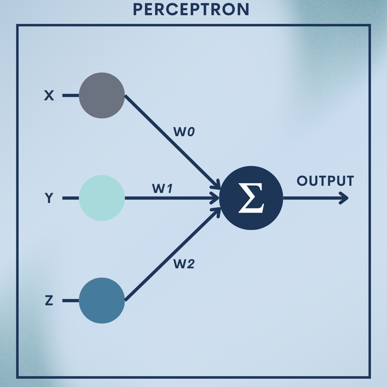
The perceptron is the simplest neuron you can build: it takes a vector of numbers, adds them up with weights, shifts by a bias, and decides yes/no via a step. Despite its simplicity, it laid the groundwork for modern neural networks. In this article you will:
- Build a perceptron from scratch and teach it to implement the AND and OR logic gates.
- Use a practical, early-style classifier on a classic dataset: detect whether a flower is Iris setosa using just two features.
- Understand exactly when perceptrons work (linearly separable data), why they fail (XOR), and how they evolved into multilayer networks.
What you’ll take away: a rock-solid grasp of the perceptron’s math, geometry, learning rule, and a reusable implementation for your code repository.
Origins and Evolution of the Perceptron
The perceptron is widely recognized as the first functional artificial neuron—a computational model inspired by the structure of biological neurons.
Its story begins long before modern deep learning.
From Biology to Mathematics: The Neuron Analogy
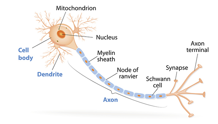
The human brain contains roughly 86 billion neurons, each receiving electrical impulses through dendrites, processing them in the soma (cell body), and transmitting signals through an axon to other neurons. The strength of connections, known as synapses, determines how signals propagate.
In the 1940s, Warren McCulloch and Walter Pitts formalized this biological process into a mathematical model: the McCulloch–Pitts (MCP) neuron.
Their 1943 paper, A Logical Calculus of the Ideas Immanent in Nervous Activity, described neurons as simple logic gates—producing binary outputs (0 or 1) based on whether the weighted sum of inputs surpassed a fixed threshold.
This was the birth of the Threshold Logic Unit (TLU)—the conceptual ancestor of the perceptron.
The Rise of Rosenblatt’s Perceptron (1957–1960s)
A decade later, Frank Rosenblatt, a psychologist and computer scientist at Cornell Aeronautical Laboratory, expanded the MCP neuron into a trainable system.
In 1957 he introduced the Perceptron, a model that could learn from examples by adjusting its internal weights according to its errors.
He physically implemented it in a device called the Mark I Perceptron, which used motors and sensors to recognize visual patterns on punch cards.
Rosenblatt’s key contribution was the Perceptron Learning Rule, an iterative algorithm that corrected weights whenever the model misclassified a sample.
This was revolutionary—it allowed machines to learn decision boundaries directly from data, rather than being explicitly programmed.
Early demonstrations showed the perceptron learning simple pattern recognition tasks, such as distinguishing triangles from squares, sparking enormous excitement across AI research.
The Fall and the AI Winter (1970s)
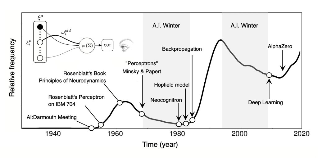
Despite the enthusiasm, the perceptron faced theoretical limits.
In 1969, Marvin Minsky and Seymour Papert published Perceptrons: An Introduction to Computational Geometry, which rigorously proved that single-layer perceptrons cannot solve non-linearly separable problems—most famously, the XOR problem.
This revelation curtailed funding for neural-network research for nearly two decades, leading to what is now known as the first AI winter.
The Revival: Multi-Layer Perceptrons and Backpropagation (1980s–Present)
The perceptron made a historic comeback in the 1980s when researchers including Rumelhart, Hinton, and Williams (1986) reintroduced the multi-layer perceptron (MLP) with the backpropagation algorithm, enabling networks to learn non-linear decision boundaries.
This innovation reignited interest in neural networks and paved the way for modern deep learning.
Today’s architectures—CNNs, RNNs, Transformers—all trace their lineage back to Rosenblatt’s simple perceptron.
Theory Deep Dive
A perceptron is essentially a mathematical abstraction of a neuron performing binary classification—deciding between two categories (e.g., spam vs not spam, setosa vs not setosa, yes vs no).
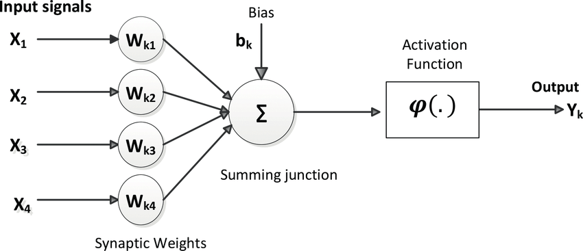
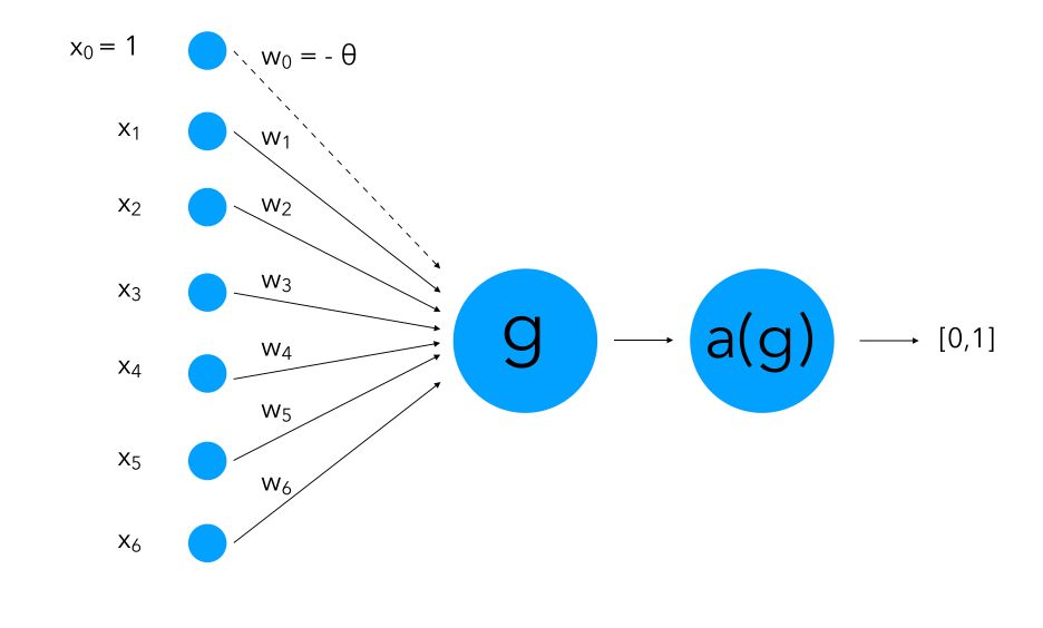
1. Inputs and Weights
Each input feature 
Each input is associated with a weight 
2. Weighted Summation
The perceptron computes a linear combination of these inputs:

where 
3. Activation Function
The summed input 

This yields a binary output, effectively deciding whether the weighted sum crosses a learned threshold.
4. Bias and Threshold
The bias (or equivalently, a negative threshold) allows the decision boundary not to be forced through the origin, improving flexibility and enabling better fits to data distributions.
5. Learning Algorithm
The Perceptron Learning Rule adjusts weights incrementally whenever an input is misclassified:


where 
This rule ensures convergence for linearly separable datasets.
Single-Layer vs Multi-Layer Perceptrons
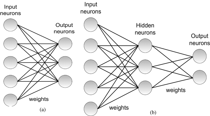
| Type | Description | Capability |
| Single-Layer Perceptron (SLP) | Consists of input features directly connected to one output neuron. | Handles only linearly separable tasks. |
| Multi-Layer Perceptron (MLP) | Stacks two or more perceptron layers with non-linear activations. | Can approximate non-linear functions and complex patterns. |
The single-layer perceptron is our focus here—it underpins the geometry and learning rule introduced next.
Its inability to model non-linear relations motivated deeper architectures and activation functions beyond the step function (e.g., sigmoid, ReLU).
Why the Perceptron Matters
- Foundation of Neural Networks: Every deep-learning neuron today—no matter how complex—still performs a weighted summation followed by a non-linear activation.
- Gateway to Learning Theory: The perceptron introduced concepts such as weights, bias, activation functions, and learning rules that form the backbone of all neural-network training.
- Understanding Linear Separability: It makes tangible the notion of decision boundaries and classification geometry.
- Historical Significance: Its rise, fall, and rebirth encapsulate the entire philosophical arc of AI research—from symbolic logic to statistical learning and connectionism.
Toy Problem – Logic Gates (AND and OR)
Data Snapshot
We will use the standard truth tables:
AND Gate
| x1 | x2 | y |
|---|---|---|
| 0 | 0 | 0 |
| 0 | 1 | 0 |
| 1 | 0 | 0 |
| 1 | 1 | 1 |
OR Gate
| x1 | x2 | y |
|---|---|---|
| 0 | 0 | 0 |
| 0 | 1 | 1 |
| 1 | 0 | 1 |
| 1 | 1 | 1 |
Both are linearly separable. XOR, by contrast, is not.
Step 1: Imports and datasets
Creates the input matrices and binary labels for AND and OR.
import numpy as np

# AND dataset
X_and = np.array([[0,0],[0,1],[1,0],[1,1]], dtype=float)
y_and = np.array([0,0,0,1], dtype=int)

# OR dataset
X_or = np.array([[0,0],[0,1],[1,0],[1,1]], dtype=float)
y_or = np.array([0,1,1,1], dtype=int)
Step 2: Perceptron class (0/1 labels)
Implements the perceptron with bias via augmentation and a step activation.
class Perceptron01:
    def __init__(self, lr=0.1, epochs=20, random_state=0):
        self.lr = lr
        self.epochs = epochs
        self.rng = np.random.default_rng(random_state)

    def _step(self, a):
        return (a >= 0).astype(int)

    def fit(self, X, y):
        n, d = X.shape
        # Bias trick: append 1 to each input; weights include bias
        Xb = np.c_[X, np.ones(n)]
        self.w = self.rng.normal(scale=0.01, size=d+1)

        for _ in range(self.epochs):
            for xi, yi in zip(Xb, y):
                yhat = self._step(np.dot(self.w, xi))
                err = yi - yhat
                if err != 0:
                    self.w += self.lr * err * xi
        return self

    def predict(self, X):
        Xb = np.c_[X, np.ones(len(X))]
        return self._step(Xb @ self.w)
Step 3: Train & test on AND
Trains on the AND table and prints predictions and learned parameters.
pp_and = Perceptron01(lr=0.1, epochs=20, random_state=42).fit(X_and, y_and)
pred_and = pp_and.predict(X_and)
print("AND predictions:", pred_and)
print("AND learned weights (including bias):", pp_and.w)
Step 4: Train & test on OR
Repeats training for the OR gate.
pp_or = Perceptron01(lr=0.1, epochs=20, random_state=42).fit(X_or, y_or)
pred_or = pp_or.predict(X_or)
print("OR predictions:", pred_or)
print("OR learned weights (including bias):", pp_or.w)
Step 5: Try changing hyperparameters (optional exploration)
Shows how learning rate and epochs influence the final separating hyperplane.
pp_fast = Perceptron01(lr=0.5, epochs=5).fit(X_and, y_and)
print("Faster training weights (AND):", pp_fast.w)
Quick Reference: Full Code
import numpy as np

X_and = np.array([[0,0],[0,1],[1,0],[1,1]], dtype=float)
y_and = np.array([0,0,0,1], dtype=int)

X_or  = np.array([[0,0],[0,1],[1,0],[1,1]], dtype=float)
y_or  = np.array([0,1,1,1], dtype=int)

class Perceptron01:
    def __init__(self, lr=0.1, epochs=20, random_state=0):
        self.lr = lr; self.epochs = epochs
        self.rng = np.random.default_rng(random_state)
    def _step(self, a): return (a >= 0).astype(int)
    def fit(self, X, y):
        n, d = X.shape
        Xb = np.c_[X, np.ones(n)]
        self.w = self.rng.normal(scale=0.01, size=d+1)
        for _ in range(self.epochs):
            for xi, yi in zip(Xb, y):
                yhat = self._step(np.dot(self.w, xi))
                self.w += self.lr * (yi - yhat) * xi
        return self
    def predict(self, X):
        Xb = np.c_[X, np.ones(len(X))]
        return self._step(Xb @ self.w)

pp_and = Perceptron01().fit(X_and, y_and)
print("AND:", pp_and.predict(X_and))

pp_or  = Perceptron01().fit(X_or, y_or)
print("OR :", pp_or.predict(X_or))
Real‑World Application — Early Classifier (Iris Setosa Detector)
Goal. Emulate an early pattern recognition task: decide if a flower is Iris setosa based on two handcrafted features. The setosa class is well separated in the classic Iris dataset, making it ideal for a perceptron.
Step 1: Load data and prepare labels
Loads Iris, selects petal features, and creates a binary label for setosa.
from sklearn.datasets import load_iris
import numpy as np
import pandas as pd

iris = load_iris()
X_all = iris.data    # columns: [sepal length, sepal width, petal length, petal width]
y_all = iris.target  # 0=setosa, 1=versicolor, 2=virginica

# Use two features strongly separating setosa
feat_idx = [2, 3]  # petal length, petal width
X = X_all[:, feat_idx]
y = (y_all == 0).astype(int)  # 1 if setosa, else 0

df = pd.DataFrame(X, columns=[iris.feature_names[i] for i in feat_idx])
df["is_setosa"] = y
print(df.head())
Data snapshot discussion.
- petal length (cm) and petal width (cm) for setosa are typically much smaller than the other species, creating near-perfect linear separability.
- The printed
head()shows the schema and typical ranges; expect values ~1–2 cm for setosa petal length/width vs larger for others.
Step 2: Train/test split and (optional) scaling
Splits the data and standardizes features for stable, faster training.
from sklearn.model_selection import train_test_split
from sklearn.preprocessing import StandardScaler

X_train, X_test, y_train, y_test = train_test_split(
    X, y, test_size=0.25, random_state=42, stratify=y
)

scaler = StandardScaler()
X_train_s = scaler.fit_transform(X_train)
X_test_s  = scaler.transform(X_test)
Step 3: Train a scikit-learn Perceptron
Fits a perceptron to the standardized features.
from sklearn.linear_model import Perceptron

clf = Perceptron(max_iter=1000, eta0=0.1, random_state=42, tol=1e-3)
clf.fit(X_train_s, y_train)

print("Weights:", clf.coef_, "Bias:", clf.intercept_)
Step 4: Evaluate performance
Reports accuracy and how predictions distribute across classes.
from sklearn.metrics import accuracy_score, confusion_matrix, classification_report

y_pred = clf.predict(X_test_s)

print("Accuracy:", accuracy_score(y_test, y_pred))
print("Confusion matrix:\n", confusion_matrix(y_test, y_pred))
print(classification_report(y_test, y_pred, target_names=["not_setosa","setosa"]))
Step 5: (Optional) Visualize decision boundary
Shows a straight line separating setosa from the other classes.
import matplotlib.pyplot as plt
import numpy as np

# Plot standardized training data
plt.scatter(X_train_s[:,0], X_train_s[:,1], c=y_train, edgecolors="k")
# Decision boundary: w1*x + w2*y + b = 0 -> y = -(w1/w2)x - b/w2
w = clf.coef_[0]; b = clf.intercept_[0]
xx = np.linspace(X_train_s[:,0].min()-1, X_train_s[:,0].max()+1, 200)
yy = -(w[0]/w[1])*xx - b/w[1]
plt.plot(xx, yy)
plt.xlabel("petal length (std)")
plt.ylabel("petal width (std)")
plt.title("Perceptron decision boundary: setosa vs not-setosa")
plt.show()
Quick Reference: Full Code
from sklearn.datasets import load_iris
from sklearn.model_selection import train_test_split
from sklearn.preprocessing import StandardScaler
from sklearn.linear_model import Perceptron
from sklearn.metrics import accuracy_score, confusion_matrix, classification_report

iris = load_iris()
X = iris.data[:, [2,3]]                 # petal length, petal width
y = (iris.target == 0).astype(int)      # setosa vs not-setosa

X_train, X_test, y_train, y_test = train_test_split(
    X, y, test_size=0.25, random_state=42, stratify=y
)

scaler = StandardScaler()
X_train_s = scaler.fit_transform(X_train)
X_test_s  = scaler.transform(X_test)

clf = Perceptron(max_iter=1000, eta0=0.1, random_state=42, tol=1e-3)
clf.fit(X_train_s, y_train)

y_pred = clf.predict(X_test_s)
print("Accuracy:", accuracy_score(y_test, y_pred))
print("Confusion matrix:\n", confusion_matrix(y_test, y_pred))
print(classification_report(y_test, y_pred, target_names=["not_setosa","setosa"]))
Strengths & Limitations
Strengths
- Simplicity & speed: Minimal parameters, very fast to train and predict.
- Interpretability: Weight signs/magnitudes directly indicate feature influence.
- Theoretical guarantee (separable data): Converges to a separator in finite steps.
Limitations
- Linear separability required: Fails on XOR-type patterns and overlapping classes.
- Hard decisions: Step output prevents probabilistic confidence and smooth optimization.
- Sensitive to scaling & outliers: Feature magnitudes and mislabeled points can hinder learning.
Final Notes
You learned the mathematics, geometric intuition, and learning dynamics of the perceptron, implemented it from scratch for AND/OR, and applied an industrially relevant, early-style binary classifier on a real dataset.
This foundation prepares you to appreciate why modern neural networks stack neurons and use differentiable activations: to go beyond linear separability.
Next Steps for You:
XOR with a hidden layer: Implement a two-layer network (an MLP) to solve XOR and see how nonlinearity emerges from composition.
Perceptron vs Logistic Regression vs SVM: Compare decision boundaries, training speed, and robustness on the Iris binary task.
Feature engineering exercise: Create two handcrafted features for a simple domain (e.g., email metadata) and test perceptron separability.
References
[1] F. Rosenblatt, “The Perceptron: A Probabilistic Model for Information Storage and Organization in the Brain,” Psychological Review, vol. 65, no. 6, pp. 386–408, 1958.
[2] M. Minsky and S. Papert, Perceptrons: An Introduction to Computational Geometry, MIT Press, 1969.
[3] A. J. Novikoff, “On Convergence Proofs on Perceptrons,” in Proc. Symposia on Math. Theory of Automata, 1962, pp. 615–622.
[4] C. M. Bishop, Pattern Recognition and Machine Learning, Springer, 2006.
[5] I. Goodfellow, Y. Bengio, and A. Courville, Deep Learning, MIT Press, 2016.
[6] T. Hastie, R. Tibshirani, and J. Friedman, The Elements of Statistical Learning, 2nd ed., Springer, 2009.
[7] Scikit-learn Developers, “Perceptron,” scikit-learn User Guide, accessed 2025.
[8] R. O. Duda, P. E. Hart, and D. G. Stork, Pattern Classification, 2nd ed., Wiley-Interscience, 2000.

Leave a comment