
Mushroom Classification → Fraud Detection
Why Random Forest?
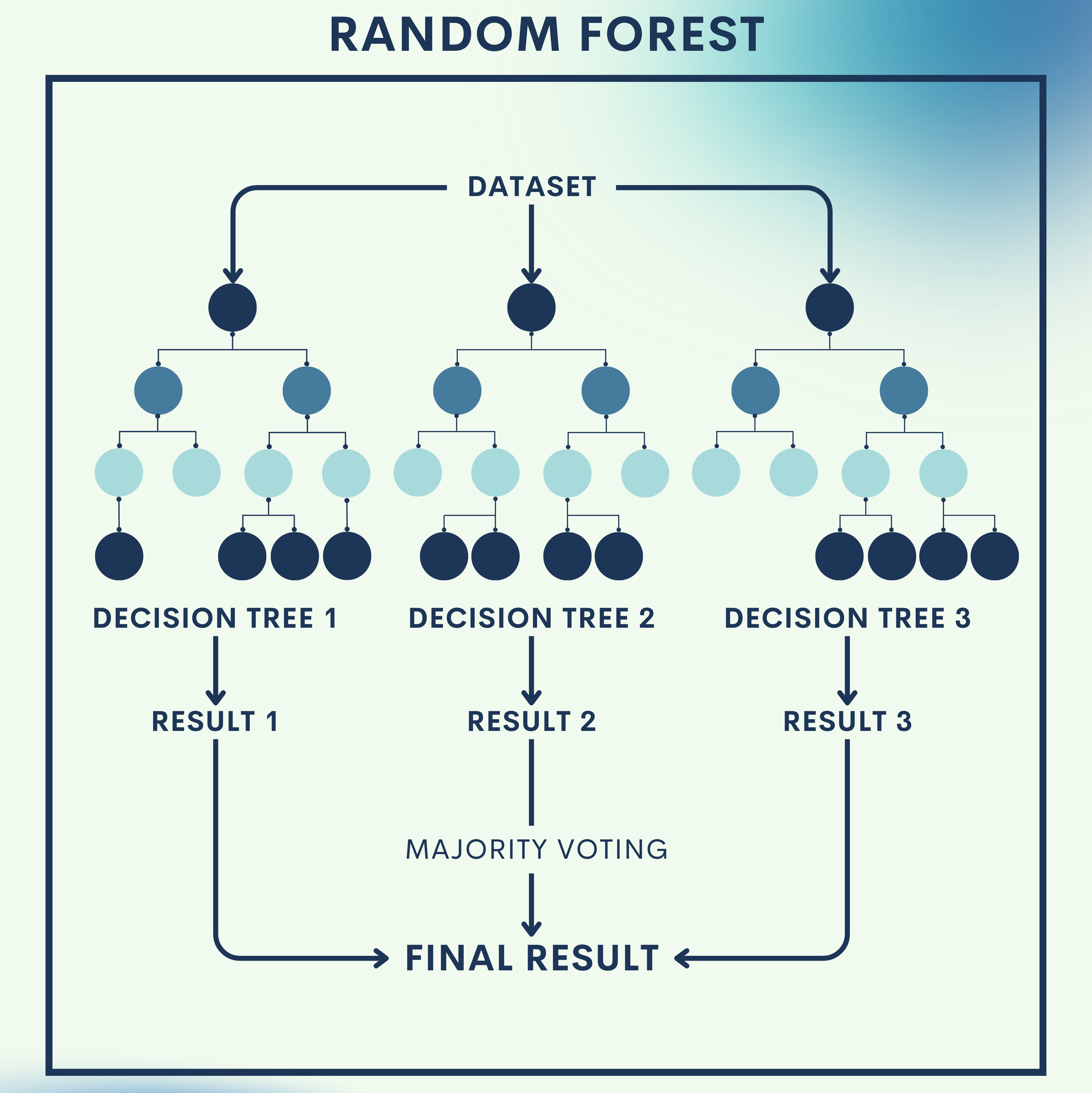
Imagine trying to decide whether a mushroom is poisonous or edible. If you ask just one person, their answer might be wrong. But if you ask a group of experts and take the majority vote, the decision is usually much more reliable.
That’s exactly what a Random Forest does: instead of relying on a single decision tree (which can easily overfit or be biased), it grows many trees on different parts of the data and then aggregates their predictions.
Practical uses include:
- Mushroom classification → predict poisonous vs. edible mushrooms.
- Fraud detection → financial institutions use Random Forests to detect suspicious transactions.
- Medical diagnosis → combining multiple factors to classify diseases.
How Ensemble Learning and Random Forest Works
Random Forest is part of ensemble learning, where multiple “weak learners” are combined to form a stronger predictor.
1. Decision Trees as Building Blocks
At the core, Random Forests rely on Decision Trees. A tree splits data based on features until it reaches a decision. But one tree alone can easily overfit.
Mathematically, a Decision Tree attempts to minimize impurity, often measured by Gini Index or Entropy:
- Entropy:
- Gini Index:


where 
2. Bagging (Bootstrap Aggregating)
Random Forests use bagging to reduce variance:
- Take multiple bootstrap samples (random sampling with replacement).
- Train a tree on each sample.
- Aggregate their results (majority vote for classification, average for regression).
Mathematically, the final prediction is:

where:
= number of trees
= prediction from the
tree
3. Random Feature Selection
To further improve diversity, each split considers only a random subset of features. This prevents trees from becoming too correlated.
Toy Problem – Mushroom Classification
We’ll use the UCI Mushroom Dataset:
- Classes: edible (e), poisonous (p)
- Features: cap shape, color, odor, gill size, etc.
Dataset Snapshot
| cap-shape | cap-color | odor | gill-size | class |
|---|---|---|---|---|
| bell | brown | none | broad | e |
| convex | yellow | foul | narrow | p |
| flat | white | spicy | narrow | p |
Step 1: Load libraries and dataset
We import needed libraries for dataset handling, model training, and evaluation.
import pandas as pd
from sklearn.model_selection import train_test_split
from sklearn.ensemble import RandomForestClassifier
from sklearn.metrics import accuracy_score, classification_report
Step 2: Load the mushroom dataset
Load the dataset and take a first look at the data.
data = pd.read_csv("mushrooms.csv")
print(data.head())
Step 3: Preprocess categorical features
Since all features are categorical, we use Label Encoding to convert them into numerical values.
from sklearn.preprocessing import LabelEncoder

encoder = LabelEncoder()
for column in data.columns:
    data[column] = encoder.fit_transform(data[column])
Step 4: Train/test split
Split the dataset into training (70%) and testing (30%).
X = data.drop("class", axis=1)
y = data["class"]

X_train, X_test, y_train, y_test = train_test_split(X, y, test_size=0.3, random_state=42)
Step 5: Train Random Forest model
Train a Random Forest with 100 decision trees.
rf = RandomForestClassifier(n_estimators=100, random_state=42)
rf.fit(X_train, y_train)
Step 6: Evaluate Performance
Check accuracy and detailed metrics (precision, recall, F1).
y_pred = rf.predict(X_test)
print("Accuracy:", accuracy_score(y_test, y_pred))
print(classification_report(y_test, y_pred))
Quick Reference: Mushroom Classification Code
import pandas as pd
from sklearn.model_selection import train_test_split
from sklearn.ensemble import RandomForestClassifier
from sklearn.metrics import accuracy_score, classification_report
from sklearn.preprocessing import LabelEncoder

# Load dataset
data = pd.read_csv("mushrooms.csv")

# Encode categorical features
encoder = LabelEncoder()
for column in data.columns:
    data[column] = encoder.fit_transform(data[column])

# Split data
X = data.drop("class", axis=1)
y = data["class"]
X_train, X_test, y_train, y_test = train_test_split(X, y, test_size=0.3, random_state=42)

# Train Random Forest
rf = RandomForestClassifier(n_estimators=100, random_state=42)
rf.fit(X_train, y_train)

# Evaluate
y_pred = rf.predict(X_test)
print("Accuracy:", accuracy_score(y_test, y_pred))
print(classification_report(y_test, y_pred))
Real‑World Application — Fraud Detection
Fraud detection is a binary classification problem (fraud vs. not fraud). Random Forests are widely used because they handle high-dimensional data and noisy features well.
Step 1: Load dataset
We use the popular credit card fraud detection dataset (imbalanced data).
data = pd.read_csv("creditcard.csv")
print(data.head())
Step 2: Train/test split
Stratified split ensures class proportions are preserved.
X = data.drop("Class", axis=1)
y = data["Class"]

X_train, X_test, y_train, y_test = train_test_split(X, y, test_size=0.3, stratify=y, random_state=42)
Step 3: Train Random Forest model
We use class weights to handle imbalance and 200 trees for stability.
rf = RandomForestClassifier(n_estimators=200, class_weight="balanced", random_state=42)
rf.fit(X_train, y_train)
Step 4: Evaluate model
We evaluate using confusion matrix and ROC-AUC, which is crucial for imbalanced problems.
from sklearn.metrics import confusion_matrix, roc_auc_score

y_pred = rf.predict(X_test)
print("Confusion Matrix:\n", confusion_matrix(y_test, y_pred))
print("ROC-AUC Score:", roc_auc_score(y_test, rf.predict_proba(X_test)[:,1]))
Full Code Collection: Fraud Detection Code
import pandas as pd
from sklearn.model_selection import train_test_split
from sklearn.ensemble import RandomForestClassifier
from sklearn.metrics import confusion_matrix, roc_auc_score

# Load dataset
data = pd.read_csv("creditcard.csv")

# Split data
X = data.drop("Class", axis=1)
y = data["Class"]
X_train, X_test, y_train, y_test = train_test_split(X, y, test_size=0.3, stratify=y, random_state=42)

# Train Random Forest
rf = RandomForestClassifier(n_estimators=200, class_weight="balanced", random_state=42)
rf.fit(X_train, y_train)

# Evaluate
y_pred = rf.predict(X_test)
print("Confusion Matrix:\n", confusion_matrix(y_test, y_pred))
print("ROC-AUC Score:", roc_auc_score(y_test, rf.predict_proba(X_test)[:,1]))
Strengths & Limitations
Strengths
- Reduces overfitting compared to single decision trees.
- Works well with both categorical and numerical features.
- Handles missing data and imbalanced datasets effectively.
Limitations
- Computationally expensive with many trees.
- Less interpretable than a single decision tree.
- Requires tuning (e.g., number of trees, depth) for best performance.
Final Notes
IIn this tutorial, we saw how Random Forests combine the wisdom of multiple trees to produce robust predictions. From a simple mushroom classification problem to detecting fraudulent transactions in financial data, Random Forests demonstrate their power across domains.
They provide a balance between accuracy and robustness, making them a go-to algorithm for many practitioners.
Next Steps for You:
Explore Gradient Boosting and XGBoost – more advanced ensemble methods.
Learn about model interpretability tools (SHAP, LIME) to explain Random Forest predictions.
References
[1] L. Breiman, “Random Forests,” Machine Learning, vol. 45, no. 1, pp. 5–32, 2001.
[2] T. Hastie, R. Tibshirani, J. Friedman, The Elements of Statistical Learning, Springer, 2009.
[3] A. Dal Pozzolo et al., “Calibrating Probability with Undersampling for Unbalanced Classification,” 2015 IEEE Symposium on Computational Intelligence and Data Mining, pp. 159–166.

Leave a comment