MNIST Compression → Data Visualization

Why PCA?

In the real world, data is often messy, massive, and high-dimensional. For example, every image in the MNIST dataset (handwritten digits) has 784 features (28×28 pixels). Imagine trying to visualize this data in just two dimensions—it seems impossible, right?

That’s where Principal Component Analysis (PCA) comes in. PCA is a mathematical technique that reduces the dimensionality of data while preserving as much information (variance) as possible.

• Toy Problem: We’ll apply PCA to compress MNIST digit images.
• Real-World Application: Use PCA to visualize large datasets in 2D or 3D, making it easier to spot clusters, trends, and anomalies.

Think of PCA as a way to find the essence of data—a simpler representation that keeps the important patterns intact.

How Principal Component Analysis (PCA) Works

1. What is PCA?

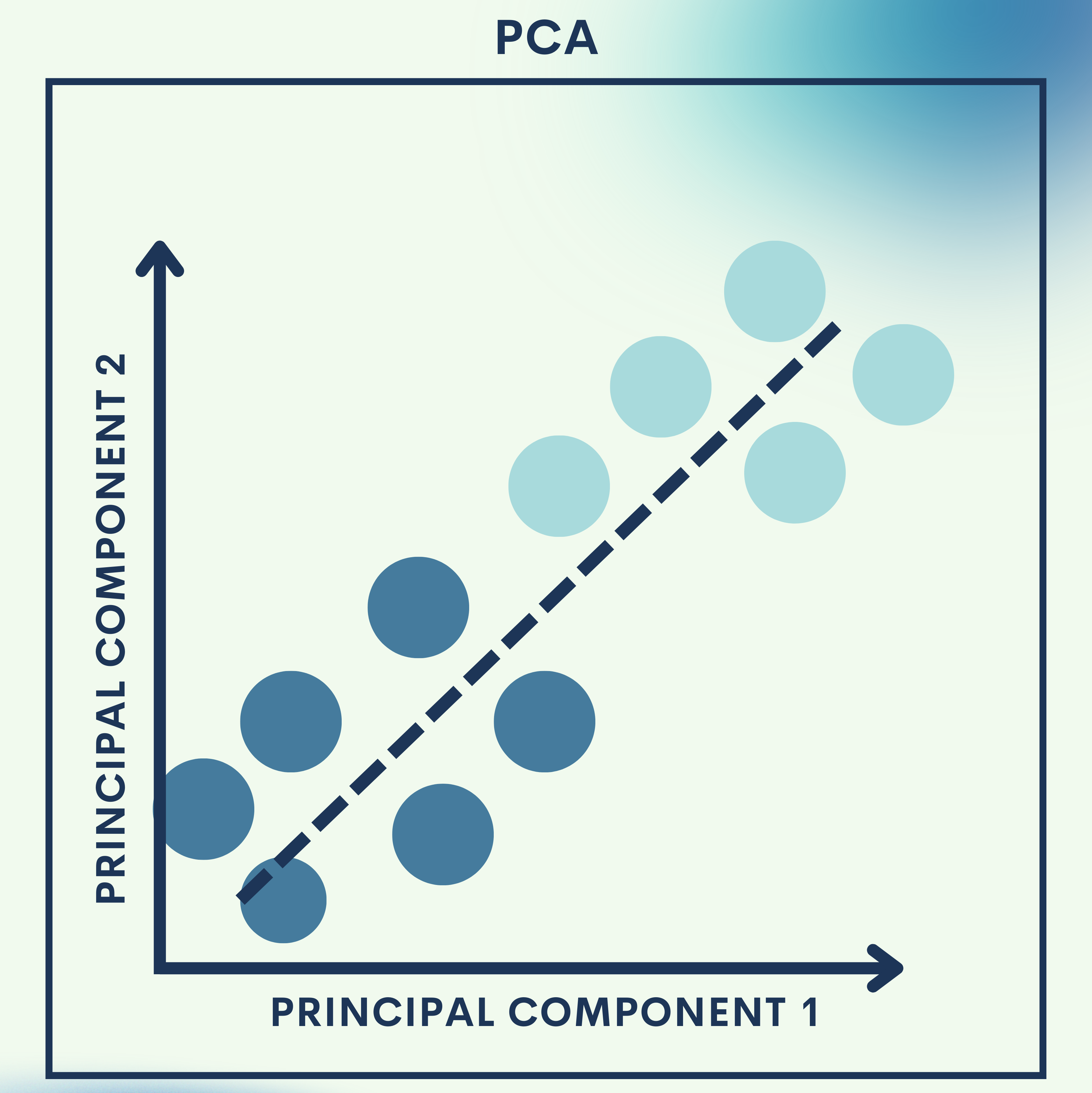
PCA is an unsupervised linear transformation method that projects data into a new coordinate system, called principal components, ordered by the amount of variance they capture.

• The first principal component captures the direction of maximum variance.
• The second principal component captures the next orthogonal direction of maximum variance.
• And so on.

This allows us to reduce dimensions while still keeping the “core” information.

2. Mathematical Foundations

Let’s say we have a dataset with samples and features.

1. Center the Data:
   Subtract the mean of each feature.
   
2. Compute the Covariance Matrix:
   
3. Eigen Decomposition:
   Solve for eigenvalues and eigenvectors:
   
   • Eigenvectors → directions of principal components.
   • Eigenvalues → amount of variance captured.
4. Projection:
   Select top eigenvectors to form matrix .
   Transform data:
   

3. Why PCA Works

• PCA finds the axes of greatest variation in the data.
• Reducing dimensions helps with speed, visualization, noise reduction, and storage efficiency.
• It’s widely used in computer vision, bioinformatics, and finance.

Toy Problem – MNIST Compression

We’ll reduce 784-dimensional images (28×28 pixels) into just 50 dimensions using PCA.

Step 1: Load the MNIST dataset

We load the MNIST dataset, which has 70,000 images with 784 features each.

from sklearn.datasets import fetch_openml
import matplotlib.pyplot as plt

# Load MNIST dataset
mnist = fetch_openml('mnist_784', version=1)
X, y = mnist.data, mnist.target.astype(int)

print("Shape of dataset:", X.shape)

Step 2: Visualize a sample digit

Displays one sample digit to remind us what the raw data looks like.

plt.imshow(X[0].reshape(28, 28), cmap="gray")
plt.title(f"Label: {y[0]}")
plt.show()

Step 3: Apply PCA for dimensionality reduction

We apply PCA to reduce from 784 features to 50.

from sklearn.decomposition import PCA

# Reduce to 50 dimensions
pca = PCA(n_components=50)
X_reduced = pca.fit_transform(X)

print("Reduced shape:", X_reduced.shape)

Step 4: Reconstruct images from reduced data

PCA compresses the image and then reconstructs it, showing how much information was preserved.

# Reconstruct back to 784 features
X_reconstructed = pca.inverse_transform(X_reduced)

# Show original vs reconstructed
fig, axes = plt.subplots(1, 2, figsize=(6, 3))
axes[0].imshow(X[0].reshape(28, 28), cmap="gray")
axes[0].set_title("Original")
axes[1].imshow(X_reconstructed[0].reshape(28, 28), cmap="gray")
axes[1].set_title("Compressed (50 dims)")
plt.show()

Quick Reference: MNIST Compression Code

from sklearn.datasets import fetch_openml
from sklearn.decomposition import PCA
import matplotlib.pyplot as plt

# Load MNIST
mnist = fetch_openml('mnist_784', version=1)
X, y = mnist.data, mnist.target.astype(int)

# PCA reduction
pca = PCA(n_components=50)
X_reduced = pca.fit_transform(X)
X_reconstructed = pca.inverse_transform(X_reduced)

# Show original vs compressed
fig, axes = plt.subplots(1, 2, figsize=(6, 3))
axes[0].imshow(X[0].reshape(28, 28), cmap="gray")
axes[0].set_title("Original")
axes[1].imshow(X_reconstructed[0].reshape(28, 28), cmap="gray")
axes[1].set_title("Compressed (50 dims)")
plt.show()

Real‑World Application — Data Visualization

Step 1: Apply PCA with 2 components

We reduce MNIST to just 2 components for visualization.

pca_2d = PCA(n_components=2)
X_pca_2d = pca_2d.fit_transform(X)

Step 2: Scatter plot of digits in 2D space

Each digit is plotted in 2D space, showing natural clusters (e.g., all “0”s group together).

import seaborn as sns

plt.figure(figsize=(10, 8))
sns.scatterplot(x=X_pca_2d[:,0], y=X_pca_2d[:,1], hue=y, 
                palette="tab10", legend=None, s=10)
plt.title("MNIST Digits Visualized with PCA")
plt.show()

Full Code Collection: Data Visualization Code

from sklearn.decomposition import PCA
import matplotlib.pyplot as plt
import seaborn as sns

# Reduce to 2D
pca_2d = PCA(n_components=2)
X_pca_2d = pca_2d.fit_transform(X)

# Scatter plot
plt.figure(figsize=(10, 8))
sns.scatterplot(x=X_pca_2d[:,0], y=X_pca_2d[:,1], hue=y, 
                palette="tab10", legend=None, s=10)
plt.title("MNIST Digits Visualized with PCA")
plt.show()

Strengths & Limitations

Strengths

• Reduces high-dimensional data to simpler forms.
• Improves visualization and interpretability.
• Helps reduce noise and redundancy.
• Speeds up training for machine learning models.

Limitations

• Only captures linear relationships (non-linear structures are ignored).
• Can lose important information if too many dimensions are reduced.
• Principal components are not always interpretable.

Final Notes

In this tutorial, we:

• Learned the theory of PCA and why it’s powerful.
• Applied PCA to compress MNIST images.
• Used PCA for data visualization to reveal digit clusters.

The key takeaway: PCA makes big, complex datasets manageable and insightful. It’s one of the most widely used tools in data science.

Next Steps for You:

Try Kernel PCA to handle non-linear data patterns.

Experiment with t-SNE or UMAP for advanced visualization beyond PCA.

References

[1] I. Jolliffe, Principal Component Analysis, Springer, 2002.
[2] C. Bishop, Pattern Recognition and Machine Learning, Springer, 2006.
[3] Y. LeCun, C. Cortes, and C. Burges, “The MNIST database of handwritten digits,” 1998.