House Price Prediction → Sales Forecasting

Why Linear Regression?

Imagine you’re a real estate agent trying to estimate house prices. You know that bigger houses usually cost more, but you want a systematic way to predict prices for new properties.

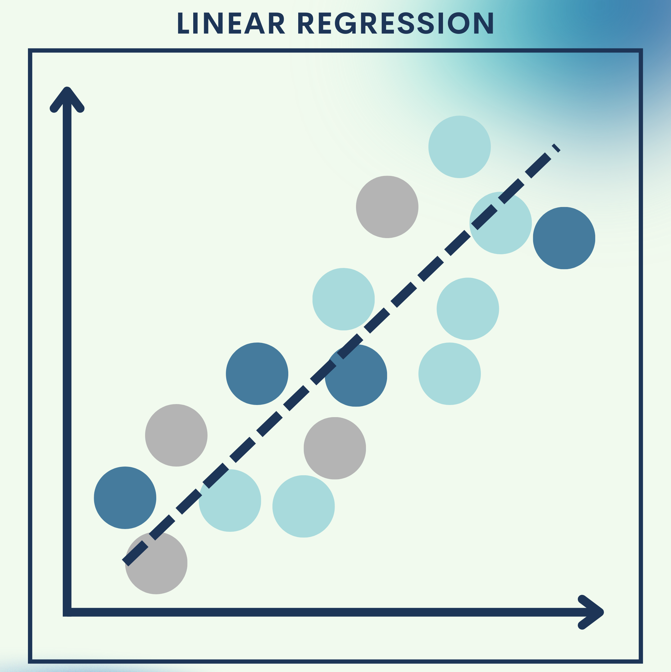
This is where Linear Regression comes in. It finds the best straight-line relationship between inputs (like house size) and outputs (like price).

In real-world business, the same principle scales up: companies use Linear Regression to forecast sales, predict demand, and understand customer trends.

How Linear Regression Works

Linear Regression is one of the oldest and most widely used algorithms in statistics and machine learning. Its main purpose is to model the relationship between one or more input variables (features) and an output variable (target).

The idea is simple: if we suspect that the output $Y$ changes linearly with the input $X$ , then we can approximate this relationship using a straight line (in simple regression) or a hyperplane (in multiple regression).

Simple Linear Regression

In the simplest case, we try to model the relationship between one input variable $X$ (for example, house size) and the output variable $Y$ (for example, house price). The model is written as:

Where:

$Y$ : the predicted value (dependent variable).
$X$ : the input feature (independent variable).
$\beta_0$ : the intercept — the baseline value of $Y$ when $X = 0$ .
$\beta_1$ : the slope — how much $latexY $ increases when $X$ increases by 1 unit.
$\epsilon$ : the error term, capturing noise and factors not explained by $X$ .

Example: If $\beta_0 = 50$ and $\beta_1 = 0.2$ , then the model predicts that for every additional square foot of house size, the price increases by $0.2$ thousand dollars.

Multiple Linear Regression

In real-world problems, one variable is rarely enough to explain the outcome. For example, house prices may depend on size, number of bedrooms, and location. To handle this, we use multiple input features:

Where:

$X_1, X_2, \dots, X_n$ are the input features (e.g., house size, number of bedrooms, distance to city).
$\beta_1, \beta_2, \dots, \beta_n$ are the coefficients (weights) showing the influence of each feature.
$\beta_0$ is still the intercept, and $\epsilon$ remains the error term.

Each coefficient $\beta_j$ can be interpreted as the marginal effect of $X_j$ on $Y$ , while holding all other variables constant.

Objective: Finding the Best Line (Training the Model)

How do we know which line (or hyperplane) fits the data best?

The most common method is Ordinary Least Squares (OLS). The idea is to choose the coefficients $\beta$ that minimize the Mean Squared Error (MSE) between actual values $Y_i$ and predicted values $\hat{Y}_i$ :

Where:

$n$ : number of training samples.
$Y_i$ : actual target value of the $latexi $-th sample.
$\hat{Y}_i$ : predicted value from the regression model.
$J(\beta)$ : the cost function we want to minimize.

Minimizing this function ensures that the regression line is as close as possible to all the data points.

Geometric Intuition

In simple regression, we are fitting a straight line in 2D space.
In multiple regression, we are fitting a flat plane (hyperplane) in higher dimensions.

The regression line is chosen such that the sum of squared vertical distances between the actual points and the line is minimized.

Why Linear Regression Works Well

Interpretability – Each coefficient tells us how much a feature contributes to the outcome.
Efficiency – It can be solved directly using matrix algebra (closed-form solution), so training is very fast.
Baseline performance – Even in complex AI projects, Linear Regression is often the first model tested because it provides a clear baseline.

Toy Problem – House Price Prediction

We’ll use a simplified dataset of houses where the size of the house (sq. ft.) predicts the price.

Dataset Snapshot

Size (sq. ft.)	Price (in $1000s)
850	150
900	170
1200	220
1500	260
1800	300

Step 1: Import Libraries

We load essential libraries for data handling, visualization, and regression modeling.

import numpy as np
import pandas as pd
import matplotlib.pyplot as plt
from sklearn.linear_model import LinearRegression

Step 2: Prepare Dataset

We structure our data into features (house size) and target (price).

# Create dataset
data = {'Size': [850, 900, 1200, 1500, 1800],
        'Price': [150, 170, 220, 260, 300]}
df = pd.DataFrame(data)

X = df[['Size']]  # feature
y = df['Price']   # target

Step 3: Train Model

We fit a Linear Regression model on the dataset.

model = LinearRegression()
model.fit(X, y)

Step 4: Make Predictions

We generate predicted prices for the given house sizes.

predictions = model.predict(X)
print(predictions)

Step 5: Visualize Results

We plot the actual data points and the regression line.

plt.scatter(X, y, color='blue', label='Actual')
plt.plot(X, predictions, color='red', linewidth=2, label='Predicted')
plt.xlabel("House Size (sq. ft.)")
plt.ylabel("Price ($1000s)")
plt.legend()
plt.show()

Quick Reference: Full Housing Price Toy Problem Code

import numpy as np
import pandas as pd
import matplotlib.pyplot as plt
from sklearn.linear_model import LinearRegression

# Dataset
data = {'Size': [850, 900, 1200, 1500, 1800],
        'Price': [150, 170, 220, 260, 300]}
df = pd.DataFrame(data)

X = df[['Size']]
y = df['Price']

# Train model
model = LinearRegression()
model.fit(X, y)

# Predictions
predictions = model.predict(X)

# Plot
plt.scatter(X, y, color='blue', label='Actual')
plt.plot(X, predictions, color='red', linewidth=2, label='Predicted')
plt.xlabel("House Size (sq. ft.)")
plt.ylabel("Price ($1000s)")
plt.legend()
plt.show()

Real‑World Application — Sales Forecasting

Retailers often want to forecast future sales based on advertising budget (TV, Radio, Online). Linear Regression can quantify how each channel contributes to sales and predict total revenue.

Step 1: Load Advertising Dataset

We define features (ad spend) and target (sales).

import pandas as pd
from sklearn.model_selection import train_test_split

# Sample advertising dataset
data = {'TV': [230, 44, 17, 151, 180],
        'Radio': [37, 39, 45, 41, 10],
        'Online': [69, 45, 69, 58, 20],
        'Sales': [22, 10, 9, 18, 15]}

df = pd.DataFrame(data)
X = df[['TV', 'Radio', 'Online']]
y = df['Sales']

Step 2: Train/Test Split

We split data into training and testing sets for evaluation.

X_train, X_test, y_train, y_test = train_test_split(X, y, test_size=0.2, random_state=42)

Step 3: Train Model

We fit Linear Regression using ad spend to predict sales.

model = LinearRegression()
model.fit(X_train, y_train)

Step 4: Evaluate Model

We evaluate how well the model predicts sales.

from sklearn.metrics import mean_squared_error, r2_score

y_pred = model.predict(X_test)
print("MSE:", mean_squared_error(y_test, y_pred))
print("R²:", r2_score(y_test, y_pred))

Full Code Collection: Full Real-World Application Code

import pandas as pd
from sklearn.model_selection import train_test_split
from sklearn.linear_model import LinearRegression
from sklearn.metrics import mean_squared_error, r2_score

# Dataset
data = {'TV': [230, 44, 17, 151, 180],
        'Radio': [37, 39, 45, 41, 10],
        'Online': [69, 45, 69, 58, 20],
        'Sales': [22, 10, 9, 18, 15]}
df = pd.DataFrame(data)

X = df[['TV', 'Radio', 'Online']]
y = df['Sales']

# Train/test split
X_train, X_test, y_train, y_test = train_test_split(X, y, test_size=0.2, random_state=42)

# Train model
model = LinearRegression()
model.fit(X_train, y_train)

# Evaluate
y_pred = model.predict(X_test)
print("MSE:", mean_squared_error(y_test, y_pred))
print("R²:", r2_score(y_test, y_pred))

Strengths & Limitations

Strengths

Simple and easy to interpret.
Fast to train, even on large datasets.
Useful as a baseline model.

Limitations

Assumes linear relationships (not always realistic).
Sensitive to outliers.
Cannot capture complex interactions between features.

Final Notes

In this tutorial, we learned:

The theory of Linear Regression and how it models relationships.
How to apply it to a toy problem (house price prediction).
How businesses use it in real-world scenarios (sales forecasting).

Linear Regression is not just academic — it’s one of the most applied AI techniques in business and research.

Next Steps for You:

Explore Polynomial Regression to model nonlinear trends.

Try applying regression to time series forecasting (e.g., monthly sales data).

References

[1] I. Goodfellow, Y. Bengio, and A. Courville, Deep Learning, MIT Press, 2016.
[2] T. Hastie, R. Tibshirani, and J. Friedman, The Elements of Statistical Learning, Springer, 2009.
[3] Scikit-learn Documentation: https://scikit-learn.org/stable/modules/linear_model.html

Linear Regression: Predicting Trends with Simple Math

Why Linear Regression?

How Linear Regression Works

Simple Linear Regression

Multiple Linear Regression

Objective: Finding the Best Line (Training the Model)

Geometric Intuition

Why Linear Regression Works Well

Toy Problem – House Price Prediction

Dataset Snapshot

Step 1: Import Libraries

Step 2: Prepare Dataset

Step 3: Train Model

Step 4: Make Predictions

Step 5: Visualize Results

Quick Reference: Full Housing Price Toy Problem Code

Real‑World Application — Sales Forecasting

Step 1: Load Advertising Dataset

Step 2: Train/Test Split

Step 3: Train Model

Step 4: Evaluate Model

Full Code Collection: Full Real-World Application Code

Strengths & Limitations

Strengths

Limitations

Final Notes

References

Leave a comment Cancel reply

Linear Regression: Predicting Trends with Simple Math

Why Linear Regression?

How Linear Regression Works

Simple Linear Regression

Multiple Linear Regression

Objective: Finding the Best Line (Training the Model)

Geometric Intuition

Why Linear Regression Works Well

Toy Problem – House Price Prediction

Dataset Snapshot

Step 1: Import Libraries

Step 2: Prepare Dataset

Step 3: Train Model

Step 4: Make Predictions

Step 5: Visualize Results

Quick Reference: Full Housing Price Toy Problem Code

Real‑World Application — Sales Forecasting

Step 1: Load Advertising Dataset

Step 2: Train/Test Split

Step 3: Train Model

Step 4: Evaluate Model

Full Code Collection: Full Real-World Application Code

Strengths & Limitations

Strengths

Limitations

Final Notes

References

Share this:

Leave a comment Cancel reply