Iris Classification → Product Recommendation

Why k-NN?

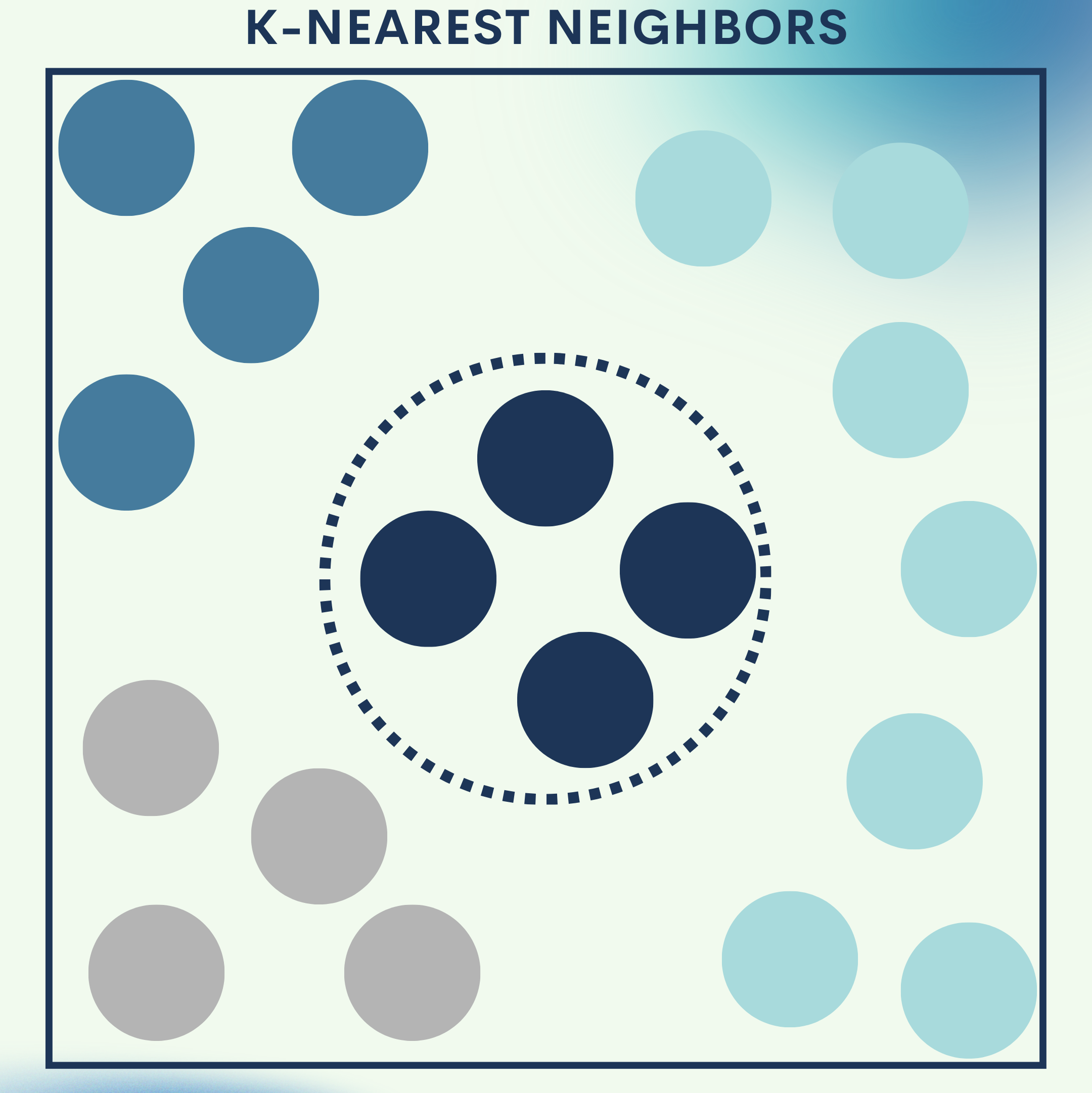
Imagine moving into a new neighborhood. To understand what life is like, you look at your closest neighbors — if most of them garden, you might start gardening; if most of them enjoy sports, you’ll likely join.

That’s what k-Nearest Neighbors (k-NN) does: it assigns labels or makes predictions for new data by checking which nearby examples it resembles the most.

How k-NN Works

k-NN is one of the simplest yet powerful instance-based learning algorithms. Instead of “training” a model with weights, it memorizes the dataset and makes predictions by comparing a new sample with existing ones.

Key Concepts:

1. Distance metric: How we define “closeness.” Common ones:
   • Euclidean distance → straight line in feature space.
   • Manhattan distance → grid-like distance (useful for sparse data).
   • Cosine similarity → angle-based similarity (common in text/recommendation).
2. Number of neighbors (k): Too small → sensitive to noise; too large → oversmooths.
3. Weights: Uniform (all neighbors equal) or distance-weighted (closer neighbors matter more).
4. Decision boundaries: Flexible, can adapt to non-linear shapes.
5. Complexity: Training is instant (just store data), but prediction can be costly for large datasets.

When to use k-NN:

• Great for small to medium datasets.
• Effective when data is fairly clean, features are meaningful, and relationships are local.
• Struggles with irrelevant features and high dimensions (curse of dimensionality).

Toy Problem – Iris Flower Classification

We’ll train a k-NN classifier to recognize three flower species based on their measurements.

Step 0: Setup & Imports

We first import all libraries required for data handling, preprocessing, modeling, and visualization. This ensures we have the right tools in place for each stage.

import numpy as np
import pandas as pd
from sklearn.datasets import load_iris
from sklearn.model_selection import train_test_split, GridSearchCV, cross_val_score
from sklearn.preprocessing import StandardScaler
from sklearn.neighbors import KNeighborsClassifier
from sklearn.metrics import accuracy_score, classification_report, confusion_matrix, ConfusionMatrixDisplay
import matplotlib.pyplot as plt

Step 1: Load Data & Snapshot

We load the Iris dataset, a balanced dataset with 150 samples. Inspecting the first few rows helps us verify structure and spot missing values.

iris = load_iris(as_frame=True)
X = iris.data
y = iris.target
df = iris.frame

print("Shape:", df.shape)
df.head()

Step 2: Train/Test Split & Scaling

We split data into training and test sets to evaluate performance fairly. Scaling is applied because k-NN relies on distance, and unscaled features can distort results.

X_train, X_test, y_train, y_test = train_test_split(
    X, y, test_size=0.25, random_state=42, stratify=y
)

scaler = StandardScaler()
X_train_s = scaler.fit_transform(X_train)
X_test_s  = scaler.transform(X_test)

Step 3: Baseline Model

We train a simple k-NN classifier with k=5 to set a baseline. This gives us a first look at the model’s performance before tuning.

knn = KNeighborsClassifier(n_neighbors=5)
knn.fit(X_train_s, y_train)
y_pred = knn.predict(X_test_s)

print("Baseline accuracy:", accuracy_score(y_test, y_pred))

Step 4: Hyperparameter Tuning

We perform grid search to find the best combination of neighbors, distance metrics, and weighting strategies. This ensures our model isn’t under- or overfitting.

param_grid = {
    "n_neighbors": list(range(1, 31)),
    "weights": ["uniform", "distance"],
    "metric": ["euclidean", "manhattan", "minkowski"]
}

grid = GridSearchCV(KNeighborsClassifier(), param_grid, scoring="accuracy", cv=5, n_jobs=-1)
grid.fit(X_train_s, y_train)

print("Best params:", grid.best_params_)
print("Best CV score:", grid.best_score_)

best_knn = grid.best_estimator_
y_pred_best = best_knn.predict(X_test_s)
print("Test accuracy:", accuracy_score(y_test, y_pred_best))

Step 5: Evaluation & Diagnostics

We generate a classification report and confusion matrix to see how well the model distinguishes between classes. This provides detailed insights beyond accuracy.

print(classification_report(y_test, y_pred_best, target_names=iris.target_names))

cm = confusion_matrix(y_test, y_pred_best)
disp = ConfusionMatrixDisplay(confusion_matrix=cm, display_labels=iris.target_names)
disp.plot()
plt.title("k-NN Confusion Matrix (Iris)")
plt.show()

Step 6: Accuracy vs. k Visualization

We plot cross-validation accuracy across different k values. This helps us see where the model performs best and avoid poor k selections.

ks = range(1, 31)
cv_scores = []

for k in ks:
    model = KNeighborsClassifier(n_neighbors=k, weights="distance")
    scores = cross_val_score(model, X_train_s, y_train, cv=5, scoring="accuracy", n_jobs=-1)
    cv_scores.append(scores.mean())

plt.plot(ks, cv_scores, marker="o")
plt.xlabel("k (neighbors)")
plt.ylabel("CV accuracy")
plt.title("Choosing k via Cross-Validation (Iris)")
plt.grid(True, linestyle="--", alpha=0.5)
plt.show()

Quick Reference: Iris Toy Problem

# --- Full Iris k-NN Pipeline ---
import numpy as np
import pandas as pd
from sklearn.datasets import load_iris
from sklearn.model_selection import train_test_split, GridSearchCV, cross_val_score
from sklearn.preprocessing import StandardScaler
from sklearn.neighbors import KNeighborsClassifier
from sklearn.metrics import accuracy_score, classification_report, confusion_matrix, ConfusionMatrixDisplay
import matplotlib.pyplot as plt

# Load data
iris = load_iris(as_frame=True)
X, y = iris.data, iris.target
df = iris.frame
print(df.head())

# Split + scale
X_train, X_test, y_train, y_test = train_test_split(X, y, test_size=0.25, random_state=42, stratify=y)
scaler = StandardScaler()
X_train_s, X_test_s = scaler.fit_transform(X_train), scaler.transform(X_test)

# Baseline model
knn = KNeighborsClassifier(n_neighbors=5)
knn.fit(X_train_s, y_train)
print("Baseline accuracy:", accuracy_score(y_test, knn.predict(X_test_s)))

# Grid search
param_grid = {"n_neighbors": list(range(1, 31)), "weights": ["uniform", "distance"], "metric": ["euclidean", "manhattan", "minkowski"]}
grid = GridSearchCV(KNeighborsClassifier(), param_grid, scoring="accuracy", cv=5, n_jobs=-1)
grid.fit(X_train_s, y_train)
best_knn = grid.best_estimator_
print("Best params:", grid.best_params_)
print("Best test acc:", accuracy_score(y_test, best_knn.predict(X_test_s)))

# Evaluation
print(classification_report(y_test, best_knn.predict(X_test_s), target_names=iris.target_names))
ConfusionMatrixDisplay.from_estimator(best_knn, X_test_s, y_test, display_labels=iris.target_names)
plt.show()

# Accuracy vs k
ks = range(1, 31)
scores = [cross_val_score(KNeighborsClassifier(n_neighbors=k, weights="distance"), X_train_s, y_train, cv=5).mean() for k in ks]
plt.plot(ks, scores, marker="o")
plt.xlabel("k"); plt.ylabel("CV Accuracy"); plt.title("Accuracy vs k"); plt.show()

Real‑World Application — Product Recommendation with k-NN

We’ll simulate a basic recommender system using item-based k-NN and cosine similarity.

Step 1: Build a User–Item Matrix

We create a toy dataset where rows are users and columns are items. Each cell indicates whether the user interacted with the item.

import pandas as pd
from sklearn.metrics.pairwise import cosine_similarity

M = pd.DataFrame(
    [
        [1, 1, 0, 0, 0],  # User A
        [1, 0, 1, 0, 0],  # User B
        [0, 1, 1, 1, 0],  # User C
        [0, 0, 1, 1, 1],  # User D
    ],
    columns=["Item_Apple", "Item_Banana", "Item_Carrot", "Item_Donut", "Item_Eclair"],
    index=["User_A", "User_B", "User_C", "User_D"]
)

Step 2: Compute Item Similarities

We calculate cosine similarity between item vectors. This tells us which items are most alike based on user behavior.

item_sim = pd.DataFrame(
    cosine_similarity(M.T),
    index=M.columns,
    columns=M.columns
)
print(item_sim.round(2))

Step 3: Recommend Similar Items

We define a function to recommend the top-k most similar items for a given product. This is the foundation of item-based collaborative filtering.

def recommend_similar_items(item_id, top_k=3):
    sims = item_sim.loc[item_id].drop(item_id).sort_values(ascending=False)
    return sims.head(top_k)

print("Similar to Item_Carrot:")
print(recommend_similar_items("Item_Carrot", top_k=3))

Full Code Collection: Product Recommendation

# --- Item-based k-NN Recommendation ---
import pandas as pd
from sklearn.metrics.pairwise import cosine_similarity

# User-item matrix
M = pd.DataFrame(
    [
        [1, 1, 0, 0, 0],
        [1, 0, 1, 0, 0],
        [0, 1, 1, 1, 0],
        [0, 0, 1, 1, 1],
    ],
    columns=["Item_Apple", "Item_Banana", "Item_Carrot", "Item_Donut", "Item_Eclair"],
    index=["User_A", "User_B", "User_C", "User_D"]
)

# Compute similarities
item_sim = pd.DataFrame(cosine_similarity(M.T), index=M.columns, columns=M.columns)

# Recommend function
def recommend_similar_items(item_id, top_k=3):
    sims = item_sim.loc[item_id].drop(item_id).sort_values(ascending=False)
    return sims.head(top_k)

print("Similar to Item_Carrot:")
print(recommend_similar_items("Item_Carrot", top_k=3))

How you’d productionize:

• Choose user‑based or item‑based k‑NN.
• Use cosine for sparse implicit data (clicks), euclidean if dense/continuous.
• For each user, score candidate items by a similarity‑weighted sum from the k nearest items they interacted with.
• Add popularity priors, time decay, and diversity filters.
• Evaluate with offline metrics (Precision@K, Recall@K, MAP, NDCG) and A/B tests.

Strengths & Limitations

Strengths

• Simplicity → Easy to understand and implement; no complex training phase.
• Flexibility → Works for both classification and regression.
• Non-parametric → Can model complex, irregular decision boundaries.
• Adaptability → Naturally supports multi-class problems without modification.
• Transparency → Predictions can be explained by showing the nearest examples.

Limitations

• Scalability → Prediction time grows with dataset size, since distances must be computed to all points.
• Curse of dimensionality → Performance degrades as the number of features grows.
• Sensitivity to noise → Outliers or mislabeled data can mislead predictions.
• Feature scaling dependency → Requires normalization/standardization to work correctly.
• Imbalanced data issues → Majority classes can dominate neighbor votes.

Final Notes

Dk-NN is one of the most intuitive algorithms in machine learning. It shows how simple ideas like “check your neighbors” can achieve strong predictive power. While it is rarely the best choice for very large or high-dimensional datasets, k-NN is excellent as a baseline model, a teaching tool, or for applications where interpretability matters.

In practice, k-NN often serves as a benchmark before deploying more sophisticated algorithms. With the right scaling, distance metric, and hyperparameters, it can still perform competitively in real-world tasks like recommendation systems, image recognition, and anomaly detection.

Next Steps for You:

Experiment with distance metrics and hyperparameters → Try different values of k and distance measures (Euclidean, Manhattan, Cosine) to see how results change. This builds intuition on how k-NN adapts to different data.

Scale to real datasets → Apply k-NN to larger problems like image classification (MNIST) or recommender systems (MovieLens). This shows its strengths and limitations in more realistic settings.

References

[1] T. Cover and P. Hart, “Nearest neighbor pattern classification,” IEEE Transactions on Information Theory, vol. 13, no. 1, pp. 21–27, 1967.
[2] scikit‑learn developers, “sklearn.neighbors.KNeighborsClassifier — scikit‑learn 1.x documentation,” Accessed: Aug. 24, 2025.
[3] R. A. Fisher, “The use of multiple measurements in taxonomic problems,” Annals of Eugenics, vol. 7, no. 2, pp. 179–188, 1936.
[4] F. Pedregosa et al., “Scikit‑learn: Machine Learning in Python,” JMLR, vol. 12, pp. 2825–2830, 2011.
[5] G. Shani and A. Gunawardana, “Evaluating recommendation systems,” in Recommender Systems Handbook, Springer, 2011.