
Play Tennis → Loan Approval Prediction
Why Decision Trees?
Think about how you make decisions in everyday life. For instance, a bank loan officer may go through a structured set of questions:
- Does the applicant have a steady job?
- If no → reject.
- If yes → move to the next question.
- Is their income high enough to cover the loan?
- If no → reject.
- If yes → move forward.
- Do they already have too many existing loans?
- If yes → reject.
- If no → approve.
This flow of yes/no questions leading to an outcome is essentially how a Decision Tree works. It’s logical, simple, and powerful — just like how we make choices every day.
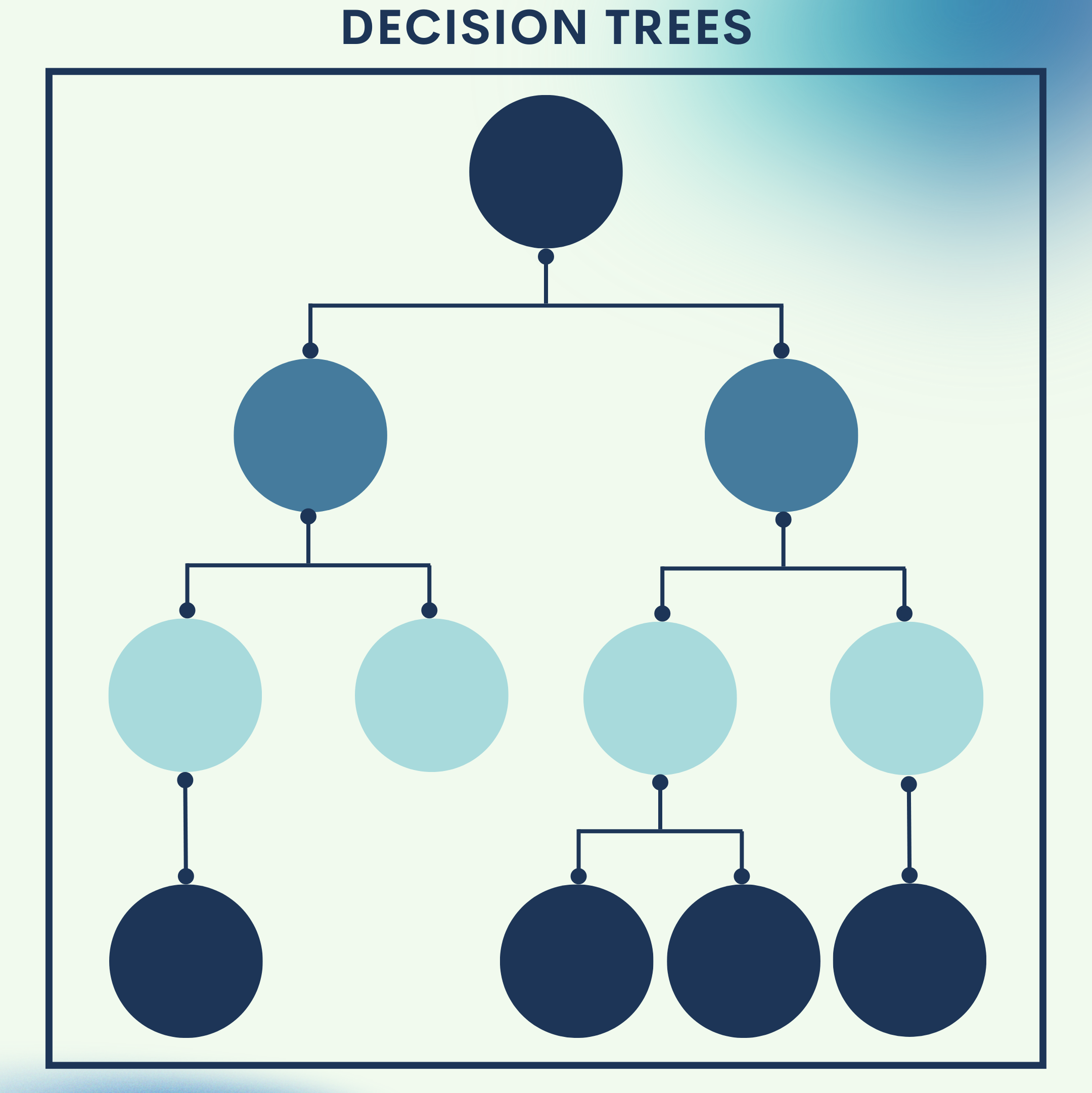
What are Decision Trees?
A Decision Tree is a supervised learning algorithm used for both classification (categorical outcomes) and regression (numerical outcomes).
- The model is structured like a tree:
- Root Node – the starting question (e.g., “Is it sunny?”).
- Internal Nodes – intermediate questions or conditions.
- Branches – possible answers (e.g., Yes/No).
- Leaf Nodes – final outcomes or decisions.
In essence, a Decision Tree works by splitting the dataset into smaller subsets based on the most informative features, until the outcome can be confidently predicted.
Why Decision Trees?
- Interpretability: Easy to understand and visualize.
- No heavy math: Works with simple logic.
- Versatility: Can handle categorical and numerical data.
- Baseline for ensembles: Forms the foundation of Random Forests and Gradient Boosting.
Toy Problem – The “Play Tennis” Dataset
This is a classic dataset used to illustrate Decision Trees. The goal is to predict whether someone will play tennis depending on the weather conditions.
Data Snapshot
| Outlook | Temperature | Humidity | Windy | PlayTennis |
|---|---|---|---|---|
| Sunny | Hot | High | False | No |
| Sunny | Hot | High | True | No |
| Overcast | Hot | High | False | Yes |
| Rain | Mild | High | False | Yes |
| Rain | Cool | Normal | False | Yes |
| Rain | Cool | Normal | True | No |
| Overcast | Cool | Normal | True | Yes |
| Sunny | Mild | High | False | No |
Goal: Given the weather conditions, predict if PlayTennis = Yes or No.
Step 1: Import libraries
What this does: Loads pandas for data handling and scikit‑learn’s DecisionTreeClassifier and export_text for training and printing the tree.
Expected output: No printed output; libraries are made available.
import pandas as pd
from sklearn.tree import DecisionTreeClassifier, export_text
Step 2: Create the dataset
What this does: Builds a small, classic “Play Tennis” dataset with weather features and a Yes/No label.
Expected output: A DataFrame with 8 rows and 5 columns (Outlook, Temperature, Humidity, Windy, PlayTennis).
data = {
    'Outlook': ['Sunny', 'Sunny', 'Overcast', 'Rain', 'Rain', 'Rain', 'Overcast', 'Sunny'],
    'Temperature': ['Hot', 'Hot', 'Hot', 'Mild', 'Cool', 'Cool', 'Cool', 'Mild'],
    'Humidity': ['High', 'High', 'High', 'High', 'Normal', 'Normal', 'Normal', 'High'],
    'Windy': [False, True, False, False, False, True, True, False],
    'PlayTennis': ['No', 'No', 'Yes', 'Yes', 'Yes', 'No', 'Yes', 'No']
}
df = pd.DataFrame(data)
df.head()
Step 3: One-hot encode the features
What this does: Converts categorical columns into numeric indicator columns (one‑hot encoding) so the tree can process them.
Expected output: A new DataFrame (df_encoded) with binary columns such as Outlook_Overcast, Outlook_Rain, Outlook_Sunny, etc.
X = pd.get_dummies(df.drop(columns='PlayTennis'))  # features
y = df['PlayTennis']                                # target label
X.head()
Step 4: Initialize and train the Decision Tree
What this does: Creates a decision tree classifier using information gain (criterion="entropy") and fits it to the encoded features and label.
Expected output: A trained model object (model). No printed output by default.
model = DecisionTreeClassifier(criterion="entropy", random_state=42)
model.fit(X, y)
Step 5: Inspect the learned rules (text view)
What this does: Prints a human‑readable set of if/else rules learned by the tree.
Expected output: A multi‑line text tree (indentation shows splits), with class: Yes/No at leaves.
tree_rules = export_text(model, feature_names=list(X.columns))
print(tree_rules)
Example of what you’ll see (structure will be similar, exact thresholds may vary):
|--- Outlook_Overcast <= 0.50
|   |--- Humidity_High <= 0.50
|   |   |--- class: Yes
|   |--- Humidity_High >  0.50
|   |   |--- class: No
|--- Outlook_Overcast >  0.50
|   |--- class: Yes
(Optional) Step 6: Make a quick prediction
What this does: Runs the trained tree on a new weather scenario to see the predicted decision.
Expected output: A single prediction: ['Yes'] or ['No'].
new_sample = pd.DataFrame([{
    'Outlook': 'Rain',
    'Temperature': 'Cool',
    'Humidity': 'Normal',
    'Windy': False
}])

new_sample_enc = pd.get_dummies(new_sample)
# Align encoded columns to training columns (fill missing with 0)
new_sample_enc = new_sample_enc.reindex(columns=X.columns, fill_value=0)

pred = model.predict(new_sample_enc)
print("Prediction for new sample:", pred.tolist())
Quick Reference: All Code Together
import pandas as pd
from sklearn.tree import DecisionTreeClassifier, export_text

# 1) Create dataset
data = {
    'Outlook': ['Sunny', 'Sunny', 'Overcast', 'Rain', 'Rain', 'Rain', 'Overcast', 'Sunny'],
    'Temperature': ['Hot', 'Hot', 'Hot', 'Mild', 'Cool', 'Cool', 'Cool', 'Mild'],
    'Humidity': ['High', 'High', 'High', 'High', 'Normal', 'Normal', 'Normal', 'High'],
    'Windy': [False, True, False, False, False, True, True, False],
    'PlayTennis': ['No', 'No', 'Yes', 'Yes', 'Yes', 'No', 'Yes', 'No']
}
df = pd.DataFrame(data)

# 2) One-hot encode features and separate target
X = pd.get_dummies(df.drop(columns='PlayTennis'))
y = df['PlayTennis']

# 3) Train decision tree (entropy = information gain)
model = DecisionTreeClassifier(criterion="entropy", random_state=42)
model.fit(X, y)

# 4) View learned rules as text
tree_rules = export_text(model, feature_names=list(X.columns))
print(tree_rules)

# 5) (Optional) Predict on a new scenario
new_sample = pd.DataFrame([{
    'Outlook': 'Rain',
    'Temperature': 'Cool',
    'Humidity': 'Normal',
    'Windy': False
}])

new_sample_enc = pd.get_dummies(new_sample)
new_sample_enc = new_sample_enc.reindex(columns=X.columns, fill_value=0)

pred = model.predict(new_sample_enc)
print("Prediction for new sample:", pred.tolist())
Real‑World Application — Loan Approval Prediction
We’ll simulate a realistic credit dataset (income, employment years, credit score, debt‑to‑income ratio, existing loans, loan amount, collateral value), train a DecisionTreeClassifier, and evaluate it.
Step 1: Import libraries
What this does: Loads core tools for data handling, modeling, and evaluation.
Expected output: No printed output.
import numpy as np
import pandas as pd

from sklearn.model_selection import train_test_split
from sklearn.tree import DecisionTreeClassifier, export_text
from sklearn.metrics import accuracy_score, classification_report, confusion_matrix
Step 2: Create (or load) a loan dataset
What this does: Generates a synthetic but realistic dataset for demo purposes. Each row is an application with features; the label Approved is derived from a rule‑of‑thumb policy with a bit of noise to mimic real life.
Expected output: A DataFrame with ~1,000 rows and 8 columns; Approved is the target.
rng = np.random.default_rng(42)
n = 1000

income = rng.normal(loc=35000, scale=12000, size=n).clip(8000, 120000)                    # yearly
employment_years = rng.integers(low=0, high=20, size=n)                                   # years
credit_score = rng.normal(loc=680, scale=70, size=n).clip(300, 850)                       # FICO-like
dti = rng.normal(loc=0.35, scale=0.15, size=n).clip(0.05, 0.95)                           # debt-to-income
existing_loans = rng.integers(low=0, high=8, size=n)                                      # count
loan_amount = rng.normal(loc=15000, scale=8000, size=n).clip(1000, 80000)                 # request
collateral_value = (loan_amount * rng.normal(loc=0.6, scale=0.25, size=n)).clip(0, 200000)
collateral_ratio = (collateral_value / loan_amount).clip(0, 5.0)

# Rule-of-thumb policy (for ground truth) + noise
score = (
    (credit_score >= 680).astype(int)
    + (income >= 25000).astype(int)
    + (employment_years >= 2).astype(int)
    + (dti <= 0.40).astype(int)
    + (existing_loans <= 3).astype(int)
    + (collateral_ratio >= 0.5).astype(int)
)
approved = (score >= 4).astype(int)

# Flip ~7% labels to simulate imperfect world
flip_mask = rng.random(n) < 0.07
approved = np.where(flip_mask, 1 - approved, approved)

df = pd.DataFrame({
    "Income": income.astype(int),
    "EmploymentYears": employment_years,
    "CreditScore": credit_score.astype(int),
    "DebtToIncome": dti,
    "ExistingLoans": existing_loans,
    "LoanAmount": loan_amount.astype(int),
    "CollateralRatio": collateral_ratio,
    "Approved": approved
})

df.head()
Step 3: Train/validation split
What this does: Splits data into train/test to fairly assess generalization.
Expected output: Four objects: X_train, X_test, y_train, y_test.
X = df.drop(columns="Approved")
y = df["Approved"]

X_train, X_test, y_train, y_test = train_test_split(
    X, y, test_size=0.2, random_state=7, stratify=y
)
Step 4: Train the Decision Tree
What this does: Fits a tree using information gain (entropy). Shallow max_depth helps avoid overfitting and keeps rules readable.
Expected output: A trained DecisionTreeClassifier in clf.
clf = DecisionTreeClassifier(
    criterion="entropy",
    max_depth=5,            # tune as needed
    min_samples_leaf=20,    # reduce overfitting
    random_state=7
)
clf.fit(X_train, y_train)
Step 5: Evaluate on the test set
What this does: Computes accuracy, confusion matrix, and a precision/recall/F1 breakdown.
Expected output: An accuracy number (e.g., ~0.85–0.95 for this synthetic data), a 2×2 confusion matrix, and a classification report.
y_pred = clf.predict(X_test)

acc = accuracy_score(y_test, y_pred)
cm = confusion_matrix(y_test, y_pred)
report = classification_report(y_test, y_pred, digits=3)

print(f"Test Accuracy: {acc:.3f}\n")
print("Confusion Matrix:\n", cm, "\n")
print("Classification Report:\n", report)
Step 6: Inspect learned rules
What this does: Prints a human‑readable set of if/else rules the model learned—useful for explainability and audits.
Expected output: A multi‑line text tree with splits on features such as CreditScore, DebtToIncome, etc.
rules = export_text(clf, feature_names=list(X.columns))
print(rules)
Step 7: Feature importance (what mattered most)
What this does: Shows which features contributed most to splitting decisions.
Expected output: A sorted list or small table of feature importances.
feat_imp = pd.Series(clf.feature_importances_, index=X.columns).sort_values(ascending=False)
print("Feature Importances:\n", feat_imp)
(Optional) Step 8: Try a few applications
What this does: Predicts approval on a couple of hypothetical applicants to demonstrate how to use the trained model.
Expected output: Model outputs [0/1] for each row plus the probability of approval.
samples = pd.DataFrame([
    # Likely approve
    {"Income": 52000, "EmploymentYears": 5, "CreditScore": 720, "DebtToIncome": 0.28,
     "ExistingLoans": 2, "LoanAmount": 18000, "CollateralRatio": 0.8},
    # Borderline
    {"Income": 24000, "EmploymentYears": 1, "CreditScore": 660, "DebtToIncome": 0.45,
     "ExistingLoans": 4, "LoanAmount": 12000, "CollateralRatio": 0.4},
])

pred = clf.predict(samples)
proba = clf.predict_proba(samples)[:, 1]  # probability of approval
out = samples.copy()
out["PredictedApproved"] = pred
out["P(Approve)"] = proba.round(3)
print(out)
Quick Reference:
import numpy as np
import pandas as pd
from sklearn.model_selection import train_test_split
from sklearn.tree import DecisionTreeClassifier, export_text
from sklearn.metrics import accuracy_score, classification_report, confusion_matrix

# -----------------------------
# 1) Create synthetic loan dataset
# -----------------------------
rng = np.random.default_rng(42)
n = 1000

income = rng.normal(loc=35000, scale=12000, size=n).clip(8000, 120000)
employment_years = rng.integers(low=0, high=20, size=n)
credit_score = rng.normal(loc=680, scale=70, size=n).clip(300, 850)
dti = rng.normal(loc=0.35, scale=0.15, size=n).clip(0.05, 0.95)
existing_loans = rng.integers(low=0, high=8, size=n)
loan_amount = rng.normal(loc=15000, scale=8000, size=n).clip(1000, 80000)
collateral_value = (loan_amount * rng.normal(loc=0.6, scale=0.25, size=n)).clip(0, 200000)
collateral_ratio = (collateral_value / loan_amount).clip(0, 5.0)

score = (
    (credit_score >= 680).astype(int)
    + (income >= 25000).astype(int)
    + (employment_years >= 2).astype(int)
    + (dti <= 0.40).astype(int)
    + (existing_loans <= 3).astype(int)
    + (collateral_ratio >= 0.5).astype(int)
)
approved = (score >= 4).astype(int)
flip_mask = rng.random(n) < 0.07
approved = np.where(flip_mask, 1 - approved, approved)

df = pd.DataFrame({
    "Income": income.astype(int),
    "EmploymentYears": employment_years,
    "CreditScore": credit_score.astype(int),
    "DebtToIncome": dti,
    "ExistingLoans": existing_loans,
    "LoanAmount": loan_amount.astype(int),
    "CollateralRatio": collateral_ratio,
    "Approved": approved
})

# -----------------------------
# 2) Train/validation split
# -----------------------------
X = df.drop(columns="Approved")
y = df["Approved"]
X_train, X_test, y_train, y_test = train_test_split(
    X, y, test_size=0.2, random_state=7, stratify=y
)

# -----------------------------
# 3) Train Decision Tree
# -----------------------------
clf = DecisionTreeClassifier(
    criterion="entropy",
    max_depth=5,
    min_samples_leaf=20,
    random_state=7
)
clf.fit(X_train, y_train)

# -----------------------------
# 4) Evaluate
# -----------------------------
y_pred = clf.predict(X_test)
acc = accuracy_score(y_test, y_pred)
cm = confusion_matrix(y_test, y_pred)
report = classification_report(y_test, y_pred, digits=3)

print(f"Test Accuracy: {acc:.3f}\n")
print("Confusion Matrix:\n", cm, "\n")
print("Classification Report:\n", report)

# -----------------------------
# 5) Inspect rules and importances
# -----------------------------
rules = export_text(clf, feature_names=list(X.columns))
print(rules)

feat_imp = pd.Series(clf.feature_importances_, index=X.columns).sort_values(ascending=False)
print("Feature Importances:\n", feat_imp)

# -----------------------------
# 6) Predict a few applications
# -----------------------------
samples = pd.DataFrame([
    {"Income": 52000, "EmploymentYears": 5, "CreditScore": 720, "DebtToIncome": 0.28,
     "ExistingLoans": 2, "LoanAmount": 18000, "CollateralRatio": 0.8},
    {"Income": 24000, "EmploymentYears": 1, "CreditScore": 660, "DebtToIncome": 0.45,
     "ExistingLoans": 4, "LoanAmount": 12000, "CollateralRatio": 0.4},
])
pred = clf.predict(samples)
proba = clf.predict_proba(samples)[:, 1]
out = samples.copy()
out["PredictedApproved"] = pred
out["P(Approve)"] = proba.round(3)
print(out)
Strengths & Limitations
Strengths
- Human-friendly and interpretable.
- Handles both categorical and numerical data.
- Useful as a baseline ML model.
Limitations
- Can overfit small datasets (too many branches).
- Not as accurate as ensemble methods (Random Forest, XGBoost).
- Unstable — small data changes may alter the tree.
Final Notes
Decision Trees are one of the best starting points in Machine Learning because they:
- Mimic human decision-making.
- Are easy to explain and visualize.
- Form the basis of advanced ensemble models.
In this tutorial, we started with the classic “Play Tennis” dataset and scaled it to a real-world loan approval scenario. This bridge between toy problems and practical applications is what makes learning AI exciting and useful.
Next Step for You: Try building a Decision Tree on another dataset — maybe predicting Titanic survival or student exam performance. The logic is the same, just the context changes.
Reference
- [1] J. R. Quinlan, “Induction of Decision Trees,” Machine Learning, vol. 1, no. 1, pp. 81–106, 1986.
- [2] L. Breiman, J. Friedman, R. Olshen, and C. Stone, Classification and Regression Trees (CART). Wadsworth International Group, 1984.
- [3] T. Hastie, R. Tibshirani, and J. Friedman, The Elements of Statistical Learning: Data Mining, Inference, and Prediction. Springer, 2009.
- [4] S. B. Kotsiantis, “Decision Trees: A Recent Overview,” Artificial Intelligence Review, vol. 39, pp. 261–283, 2013.
- [5] S. Raschka and V. Mirjalili, Python Machine Learning, 3rd ed. Packt Publishing, 2019.
- [6] F. Pedregosa et al., “Scikit-learn: Machine Learning in Python,” Journal of Machine Learning Research, vol. 12, pp. 2825–2830, 2011.
- [7] UCI Machine Learning Repository – “Play Tennis Dataset,” [Online]. Available: https://archive.ics.uci.edu/ml/index.php
- [8] Scikit-learn Documentation – “Decision Trees,” [Online]. Available: https://scikit-learn.org/stable/modules/tree.html

Leave a comment